OpenObserve vs Elasticsearch: Benchmark at 1.1 TB Scale

TLDR

We streamed 1.1 TB of synthetic Kubernetes-format log data to both systems simultaneously on identical AWS hardware. On ingestion: Elasticsearch dropped 62% of the data due to schema mapping conflicts, throttled at 96% CPU, and used 10x more RAM. OpenObserve accepted everything, compressed it 9.5x, ran at 15% CPU, and was 87x cheaper on storage. On queries: OpenObserve won 14 out of 15 - up to 32x faster on aggregations. The one area Elasticsearch wins is COUNT(*) queries, by 1.5x.

Overview

The ELK stack has been one of the most popular logging backends for the last decade. But running Elasticsearch at scale — we're talking terabytes of daily ingestion — demands significant resources and ongoing operational effort. Tuning JVM heap, managing index mappings, handling shard rebalancing, and keeping the cluster healthy under load are all real costs that teams absorb continuously.

OpenObserve is a highly efficient alternative built for exactly this scale. It is designed to minimize storage footprint and reduce compute overhead compared to Elasticsearch — not just as a claim, but as a measurable, testable property.

To put that to the test, we ran a full performance benchmark: same AWS hardware, same 1.1 TB of Kubernetes-format log data, both systems receiving identical log streams simultaneously. The results cover storage efficiency, CPU utilization, RAM usage, and query performance.

The dataset: Log data was generated synthetically using a custom Python script based on the Kubernetes log schema from OpenObserve's sample K8s dataset. Generated logs were written to a file and forwarded through Fluent Bit to both systems simultaneously using a dual-output configuration — ensuring both Elasticsearch and OpenObserve received identical log streams at the same time. A fixed random seed (random.seed(42)) was used to ensure reproducibility — anyone running the benchmark with the same script will get identical data distribution. Total raw data sent: 1,122 GB (~1.1 TB). To replicate the benchmark yourself, check the repo: github.com/openobserve/o2-vs-elasticsearch-benchmark.

Infrastructure

Machine	Role	Instance	vCPU / RAM	Storage
bench-generator	K8s-format log generator	c5.2xlarge	8 / 16 GB	30 GB EBS
bench-elasticsearch	Elasticsearch 8.19	r7gd.2xlarge	8 / 64 GB	474 GB NVMe
bench-openobserve	OpenObserve v0.90	r7gd.2xlarge	8 / 64 GB	474 GB NVMe

Both systems ran on identical hardware. Same instance type, same RAM, same NVMe storage.

Part 1: Storage Efficiency

The Numbers

Metric	Elasticsearch	OpenObserve
Raw data sent	1,122 GB	1,122 GB
Docs accepted	487 million (38%)	1.27 billion (100%)
Docs dropped	780 million (62%)	0
Raw data accepted	~429 GB	1,122 GB
Stored on disk	375 GB	118 GB
True compression ratio	1.14x	9.5x
Disk used (actual)	375 GB / 474 GB (79%)	211 GB(indexing included) / 474 GB (44%)

Why Did Elasticsearch Drop 62% of the Data?

This is the most critical finding of the entire benchmark. Elasticsearch rejected 780 million documents - not due to hardware limits, but due to strict field type mapping conflicts.

In Kubernetes-format logs, fields like kubernetes.labels.app can appear as both a string and a nested object across different log lines from different pods. Elasticsearch locks in the field type on first write. Every subsequent document where the type differs gets rejected with a mapping conflict error.

OpenObserve accepted all 1.27 billion documents with zero configuration changes. No schema management. No mapping templates. No pre-configuration required.

What we did next: To continue the benchmark beyond this finding, we deleted the Elasticsearch indexes, explicitly set the conflicting fields (e.g. kubernetes.labels.app) to the flattened type in the mapping, and re-ingested the full dataset. The flattened type tells Elasticsearch to treat the entire field as a single flat value, bypassing the type conflict. This allowed ingestion to proceed — but it required manual intervention before a single byte of data could be reliably stored.

If you have ever run K8s at scale, you'll know Kubernetes log schemas are inherently inconsistent — different deployments, different helm chart versions, different application owners all contribute logs with varying field shapes. The generated dataset intentionally reflected this real-world variability. Elasticsearch requires upfront schema engineering every time a new field shape appears. OpenObserve handles it out of the box.

Compression Ratio at Scale

OpenObserve maintained a consistent 9.5–10x compression ratio from 10 GB all the way to 1 TB. Elasticsearch barely compressed at all, averaging 1.14x across the entire run.

Raw Data Accepted	ES Stored	O2 Stored	ES Ratio	O2 Ratio
10 GB	~10 GB	~1 GB	1x	10x
43 GB	~34 GB	~4.3 GB	1.3x	10x
150 GB	~127 GB	~15 GB	1.2x	10x
250 GB	~199 GB	~25 GB	1.3x	10x
429 GB (ES) / 1,122 GB (O2)	375 GB	118 GB	1.14x	9.5x

Part 2: CPU Utilization

Server Utilization

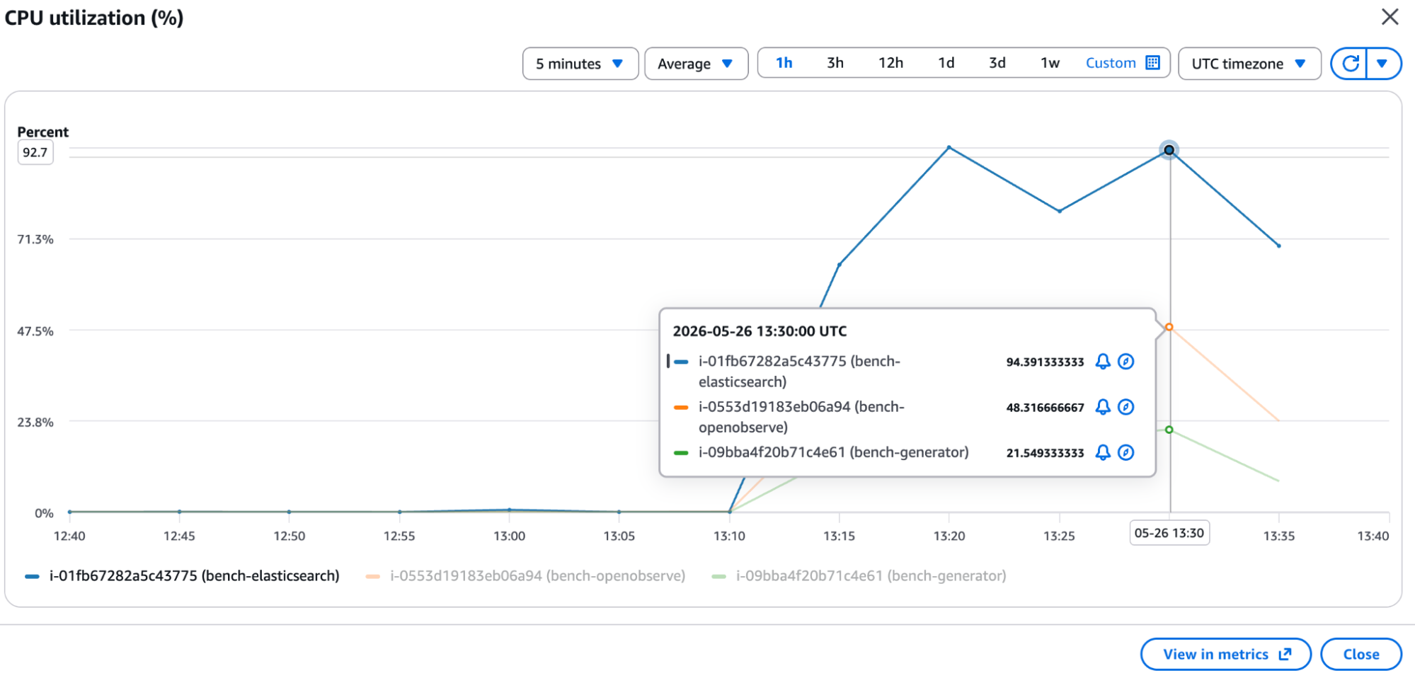
This is what the CPU graphs looked like during active ingestion. Elasticsearch (blue) climbed to ~94% and stayed there. OpenObserve (orange) held steady at ~48%.

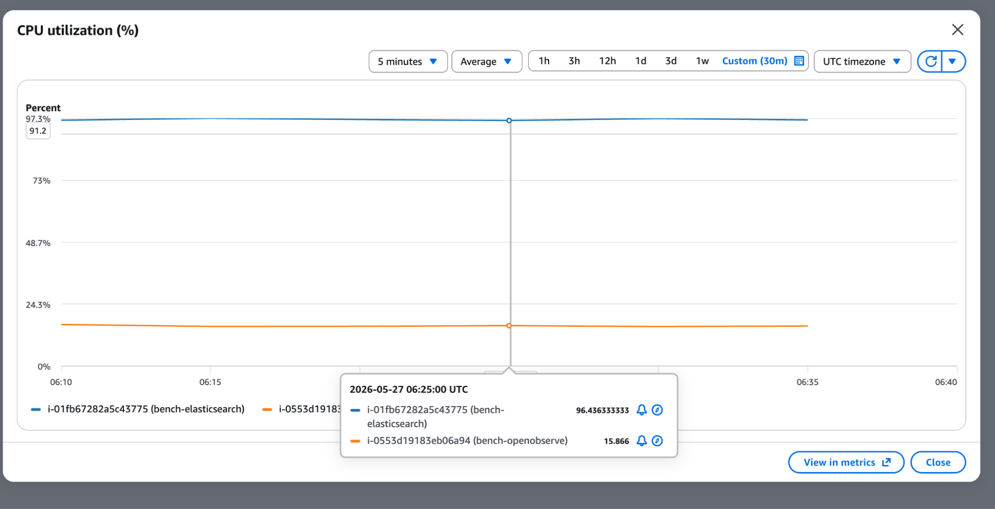
The sustained picture was even more stark. Over a 30-minute custom window, Elasticsearch sat at a flat ~96% — actively throttling. OpenObserve held at ~15%.

CPU Summary Table

Phase	Elasticsearch	OpenObserve	Advantage
Peak ingestion	95–96%	49%	2x less
Sustained ingestion	~96% (throttling)	~15%	6x less
Idle baseline	~19–20%	~3–5%	5–6x less

At 96% sustained CPU, Elasticsearch was throwing 429 (Too Many Requests) errors and slowing down ingestion. OpenObserve never came close to a resource ceiling.

Part 3: RAM Usage

Metric	Elasticsearch	OpenObserve
Total RAM	64 GB	64 GB
RAM used (peak ingestion)	19 GB	1.9 GB
RAM available	43 GB	61 GB
Difference	baseline	10x less RAM

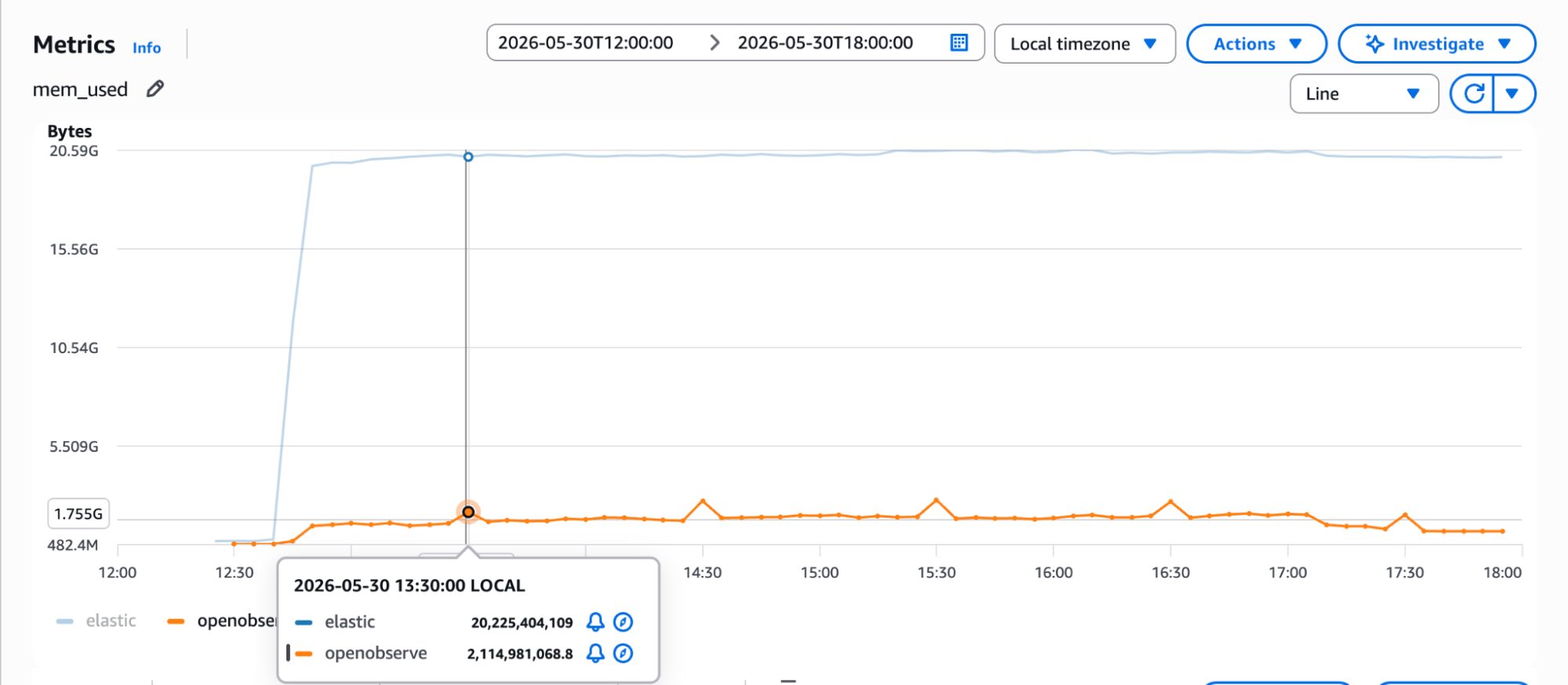
OpenObserve used 1.9 GB of RAM at peak ingestion. Elasticsearch consumed 19 GB - 10x more on the same 64 GB machine. This isn't a rounding-error difference. It has direct implications for instance sizing, cluster memory requirements, and overall infrastructure cost.

The memory metrics from AWS confirm this visually:

Part 4: Ingestion Speed

For the ingestion speed test, Elasticsearch was deliberately given an advantage: it ran on an m7gd.4xlarge (16 vCPU, 64 GB RAM, 950 GB NVMe). OpenObserve remained on the original r7gd.2xlarge (8 vCPU, 64 GB RAM, 474 GB NVMe). ES had double the CPU.

Metric	Elasticsearch	OpenObserve
Instance	m7gd.4xlarge (16 vCPU)	r7gd.2xlarge (8 vCPU)
Total docs ingested	2.07 billion	2.75 billion
Duration	8.08 hours	8.08 hours
Ingestion speed	~71,300 events/sec (16 vCPU)	~94,900 events/sec (8 vCPU)
Advantage	baseline	9x faster per CPU core

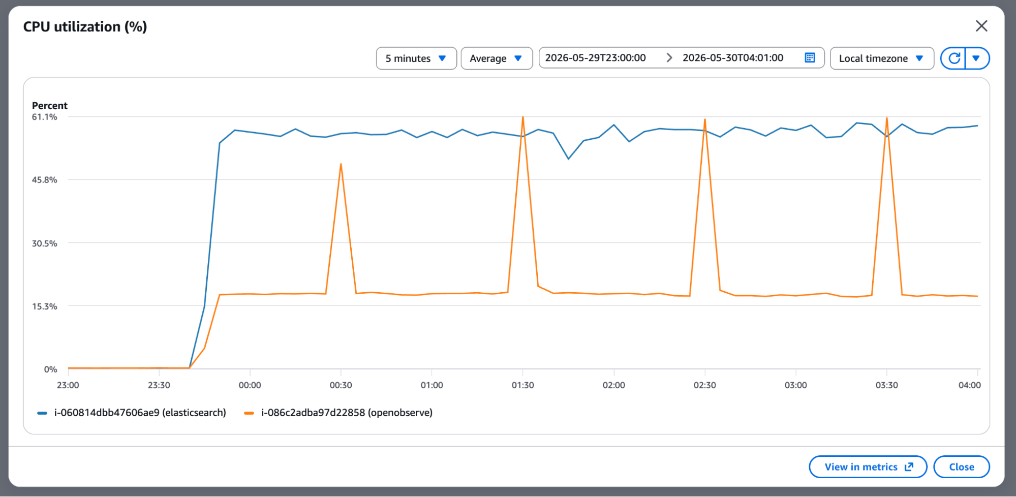
OpenObserve ingested 9x more events per second per CPU core, on half the CPU. If both ran on identical hardware, the gap would be even larger.

The AWS CPU graph for this test period shows it clearly — Elasticsearch (blue) staying elevated throughout, OpenObserve (orange) spiking briefly then running efficiently at a fraction of the CPU:

The disk write operations and network throughput charts confirm that both systems were receiving the same input - identical network ingress, but very different storage behavior:

Storage Saturation and Hardware Upgrade

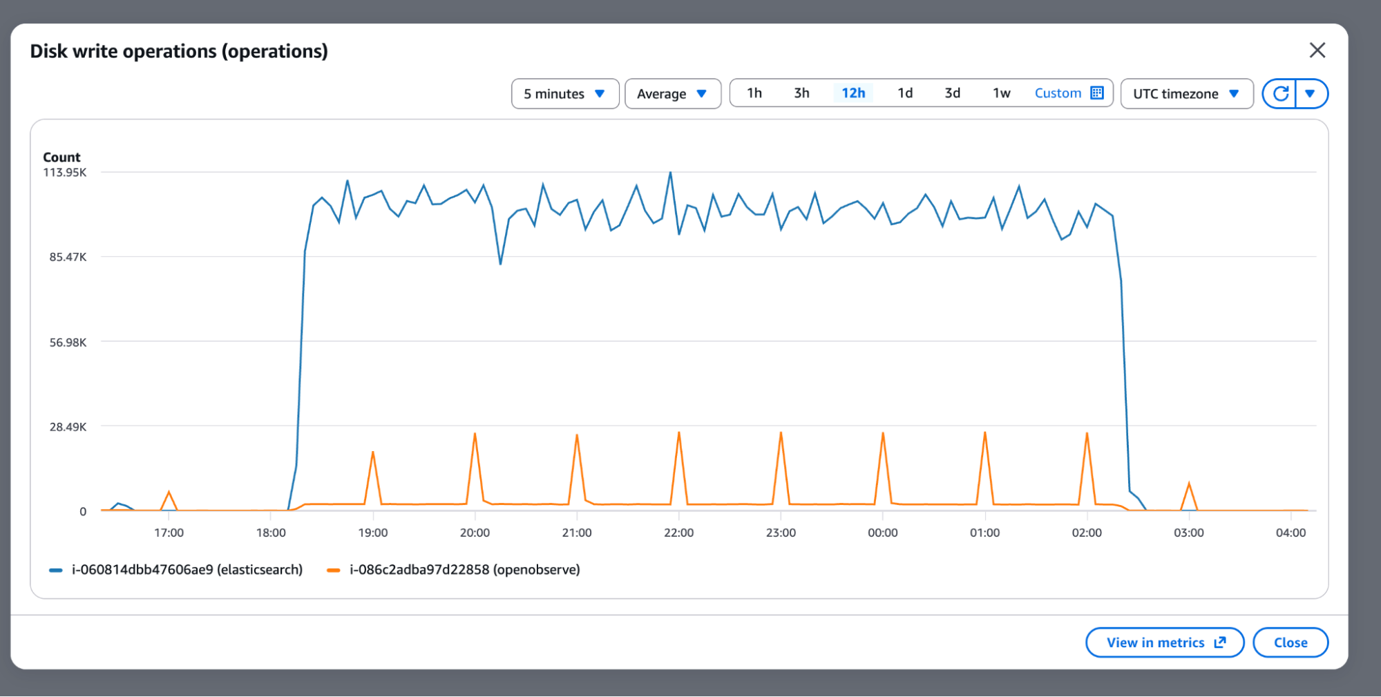
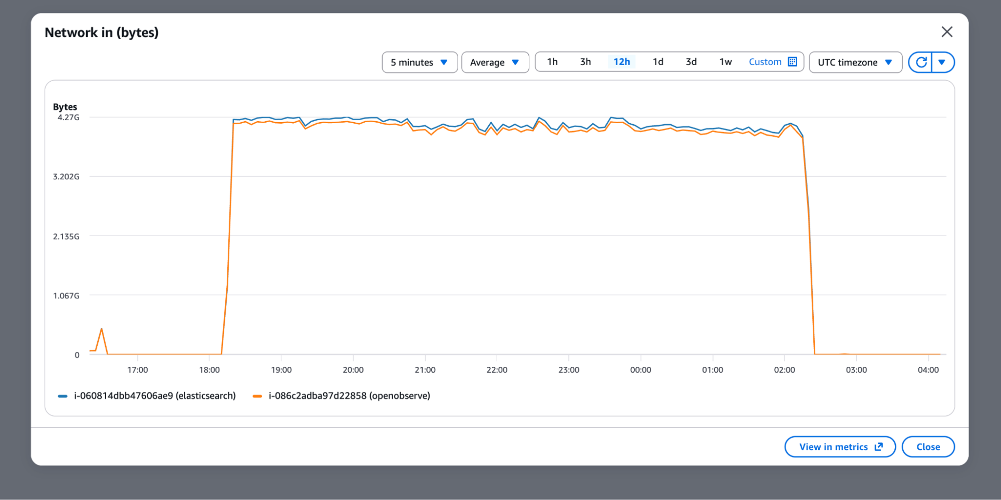
Elasticsearch exhausted the 474 GB NVMe drive during ingestion, consuming roughly 7.5x more storage than OpenObserve for the same raw workload. To continue testing without hitting disk limits mid-run, the Elasticsearch node was upgraded to an m7gd.4xlarge (16 vCPU, 884-950 GB NVMe) for the ingestion speed and query benchmarks. OpenObserve remained on the original r7gd.2xlarge throughout.

Part 6: Storage Cost Comparison

These numbers use a fair comparison: assume Elasticsearch accepts 100% of the data (ignoring the 62% drop rate from the real benchmark) and compare just the storage economics.

Assumptions:

• Elasticsearch: HA mode with 1 primary + 2 replicas = 3x replication on EBS ($0.08/GB/month)
• OpenObserve: Single copy on S3 — AWS natively replicates across 3 AZs ($0.023/GB/month)
• Raw data: 1,122 GB

	Elasticsearch	OpenObserve
Compression ratio	1.14x	9.5x
After compression	984 GB	118 GB
Replication	× 3 (HA)	× 1 (S3 native)
Total storage	2,952 GB	118 GB
Storage cost/month	$236.16	$2.71
Cost ratio	baseline	87x cheaper

At scale, storage cost is one of the largest line items in observability infrastructure. An 87x difference in storage cost on identical raw data is not marginal - it changes the economics of the entire system.

Part 7: Query Performance

All queries used in this benchmark are available on GitHub: benchmark_queries.md

To keep the benchmarking fair, OpenObserve resources were also upgraded for this test matching the same uplift given to Elasticsearch after the storage saturation event.

Test environment:

Component	Details
Elasticsearch	v8.19.16 — m7gd.4xlarge (16 vCPU, 128 GB RAM, 884 GB NVMe)
OpenObserve	v0.90.0 Enterprise —m7gd.4xlarge (16 vCPU, 128 GB RAM, 884 GB NVMe)

Full Results

Query	Type	ES Cold	O2 Cold	Cold Winner	ES Warm	O2 Warm	Warm Winner
Q01 Filter-Namespace	Simple Filter	5,549ms	38ms	✅ O2 146x	46ms	32ms	✅ O2 1.4x
Q02 Filter-Container	Simple Filter	67ms	31ms	✅ O2 2.2x	47ms	29ms	✅ O2 1.6x
Q03 Filter-Host	Simple Filter	56ms	30ms	✅ O2 1.9x	62ms	30ms	✅ O2 2.1x
Q04 Filter-Stream	Simple Filter	69ms	30ms	✅ O2 2.3x	40ms	30ms	✅ O2 1.3x
Q05 Filter-Role	Simple Filter	51ms	30ms	✅ O2 1.7x	47ms	30ms	✅ O2 1.6x
Q06 FTS-Failed	Full Text Search	748ms	30ms	✅ O2 24.9x	498ms	30ms	✅ O2 16.6x
Q07 FTS-Connection	Full Text Search	183ms	31ms	✅ O2 5.9x	187ms	30ms	✅ O2 6.2x
Q08 FTS-Scrape	Full Text Search	168ms	30ms	✅ O2 5.6x	151ms	31ms	✅ O2 4.9x
Q09 Agg-Namespace	Aggregation	3,134ms	744ms	✅ O2 4.2x	3,305ms	615ms	✅ O2 5.4x
Q10 Agg-Container	Aggregation	3,253ms	737ms	✅ O2 4.4x	3,476ms	612ms	✅ O2 5.7x
Q11 Agg-Host	Aggregation	21,239ms	951ms	✅ O2 22.3x	21,590ms	678ms	✅ O2 31.8x
Q12 Filter+Agg	Combined	722ms	556ms	✅ O2 1.3x	812ms	478ms	✅ O2 1.7x
Q13 FTS+Filter	Combined	480ms	31ms	✅ O2 15.5x	455ms	31ms	✅ O2 14.7x
Q14 Count-All	Heavy	35ms	55ms	✅ ES 1.6x	36ms	54ms	✅ ES 1.5x
Q15 Agg-Role	Heavy	3,544ms	713ms	✅ O2 5.0x	3,568ms	602ms	✅ O2 5.9x

Score: OpenObserve wins 14/15 on both cold and warm cache.

Summary by Query Type

Query Type	ES Cold Avg	O2 Cold Avg	Cold Winner	ES Warm Avg	O2 Warm Avg	Warm Winner
Simple Filter	1,158ms	32ms	O2 36x	48ms	30ms	O2 1.6x
Full Text Search	366ms	30ms	O2 12x	279ms	30ms	O2 9.3x
Aggregation	9,209ms	811ms	O2 11x	9,457ms	635ms	O2 14.9x
Combined	601ms	294ms	O2 2x	634ms	255ms	O2 2.5x
Heavy	1,790ms	384ms	O2 4.7x	1,802ms	328ms	O2 5.5x

Key Query Observations

Full text search is where the gap is most dramatic. OpenObserve's columnar storage with inverted index handles substring search 5–25x faster cold and 5–17x faster warm. The Q06 result (748ms vs 30ms cold) shows how badly ES struggles with match queries on large datasets at cold cache.

Aggregations are the other standout. Q11 (high-cardinality host field, 200 unique values) ran in 21 seconds on Elasticsearch. OpenObserve returned 951ms cold and 678ms warm. That's a 31.8x warm speedup for a query type that shows up constantly in real dashboards. Columnar format is purpose-built for GROUP BY operations.

ES aggregations show no caching benefit -warm times were nearly identical to cold (Q11: 21,239ms cold vs 21,590ms warm). ES result cache simply wasn't effective for these aggregation shapes. O2 showed clear improvement on warm cache across all aggregation queries.

Elasticsearch wins only COUNT(*). Pre-computed document counts give it a 1.5–1.6x edge on pure count queries. This is the one area where ES's inverted index architecture has a structural advantage.

Summary

Metric	Elasticsearch	OpenObserve	Advantage
Storage compression	1.14x	9.5x	✅ 8.3x better compression
Disk used	375 GB	118 GB	✅ 3.2x smaller footprint
RAM (peak ingestion)	19 GB	1.9 GB	✅ 10x less RAM
CPU sustained	96%	15%	✅ 6x less CPU
Data accepted	38%	100%	✅ 2.6x more data ingested
Schema flexibility	Manual mapping	Automatic	✅ Zero config
Storage cost/month	$236.16	$2.71	✅ 87x cheaper
Query performance	baseline	14/15 queries faster	✅ Clear winner
Ingestion speed	71,300 ev/sec (16 vCPU)	94,900 ev/sec (8 vCPU)	✅ 9x faster per CPU core

Workload Recommendations

Workload	Recommended
Full text / substring search	OpenObserve (5–25x faster)
Aggregations / GROUP BY	OpenObserve (4–32x faster)
Simple field filters	OpenObserve (1.3–146x faster)
Combined FTS + filter	OpenObserve (15x faster)
COUNT(*) queries	Elasticsearch (1.5x faster)
K8s-format logs (mixed schema)	OpenObserve (ES drops 62%)
Cost-sensitive observability at scale	OpenObserve (87x cheaper storage)

Conclusion

This benchmark started as a validation exercise. It ended up revealing something more significant than performance numbers: Elasticsearch has fundamental architectural mismatches with Kubernetes-format log workloads at scale.

The 62% document drop rate isn't a tuning problem — it's what happens when a row-oriented search engine with strict schema enforcement meets the schema variability inherent in Kubernetes-format logs. The 96% CPU during sustained ingestion means Elasticsearch is operating at the edge of its capacity on hardware that OpenObserve uses at 15%.

OpenObserve's columnar storage, automatic schema handling, and S3-native architecture produce results that aren't marginal improvements , they're order-of-magnitude differences on the metrics that matter most: storage cost, CPU headroom, RAM consumption, query latency on aggregations and full-text search, and the fundamental reliability of actually accepting all your data.

The one area where Elasticsearch retains an edge COUNT(*) queries is real but narrow (1.5x). For the overwhelming majority of log analytics workloads, the numbers in this report tell a clear story.