The Query Tantivy Couldn't Save in OpenObserve: 2.6s to 89ms for Random High-Cardinality Lookups

Last time, two config changes took a count query from 49 seconds to 2 seconds.

But that win has a quiet asterisk. For one specific shape of query — a random high-cardinality lookup, like searching by trace_id — neither of those changes does anything. The query still scans every file. That's the query this post is about.

Previous in series

How we cut a query from 49 seconds to 2 seconds. Raise ZO_COMPACT_MAX_FILE_SIZE from 1 GB to 10 GB; turn on the tantivy footer cache. The same 2 TB dataset, the same count query, ~25× faster. If you haven't read it, that's the story of how we collapsed an order of magnitude of S3 round trips. This post is the follow-up — what happens when even that isn't enough.

The query that didn't get fixed

The first post's win lived in a particular regime: filtered queries on fields where the filter is selective and the index can range-prune. Once compact files were big and tantivy footers were cached, the work shrank to "open a few files, hit the index, read the matching rows." A clean order-of-magnitude improvement.

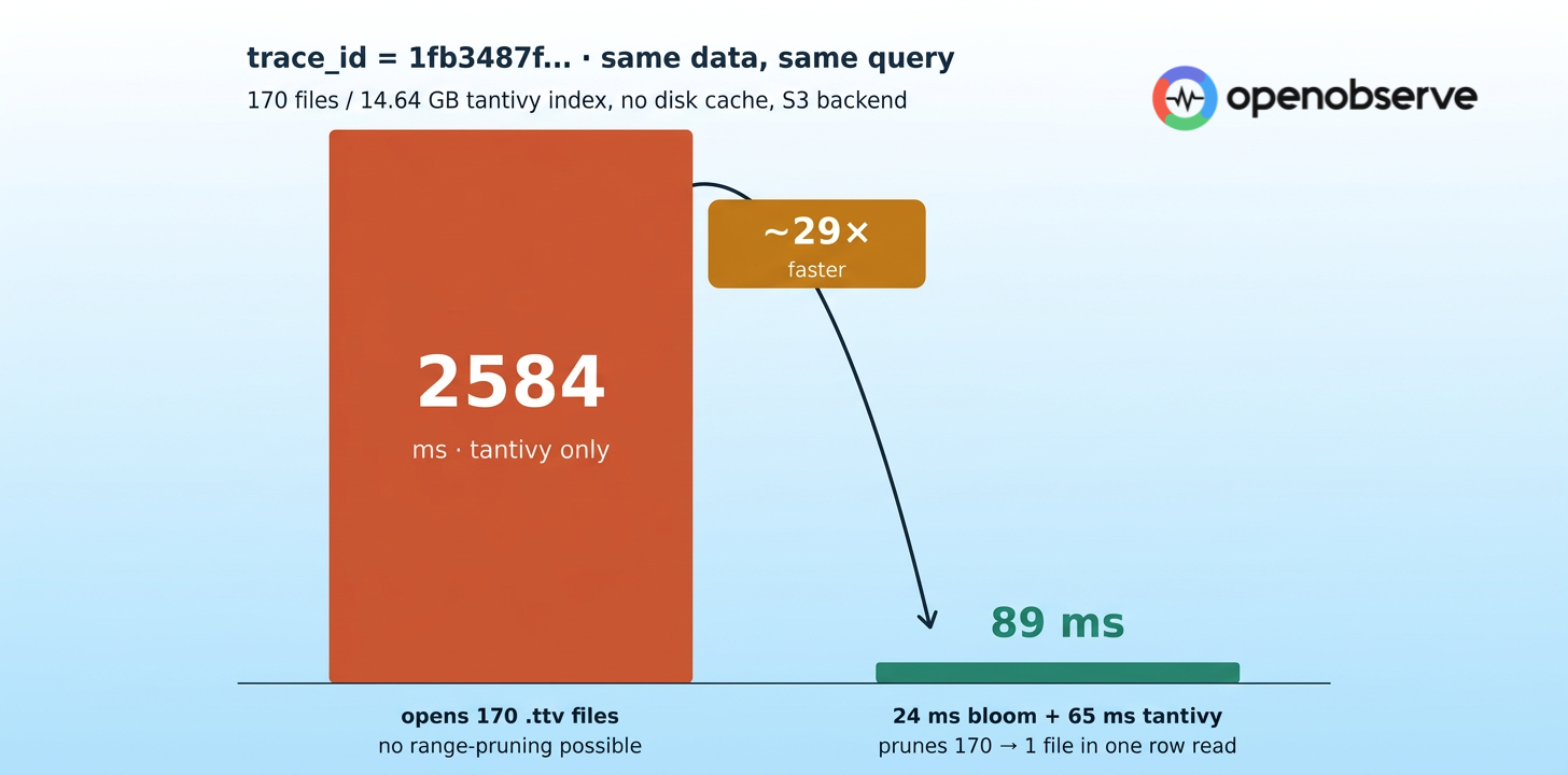
Then we ran a different query. A single matching trace_id over a stream called benchtest — 170 parquet files for the hour, ~14.6 GB of tantivy index files, no disk cache. The query that, by intuition, should be the easiest: needle in a haystack, one needle, exactly one matching row.

It took 2,584 milliseconds.

That number is not catastrophic in isolation. But it's not what you'd expect from an indexed lookup that returns one row. And nothing in the previous post's toolkit fixed it. Bigger compact files? Doesn't help — there's nothing to compact away. Footer cache? Already on. We were squarely in the "open the index" stage, and the index opens were the cost.

The reason is mechanical, and once you see it, the whole layer below this post falls into place.

Why tantivy can't range-prune a random ID

Tantivy keeps a small sparse index per .ttv file — it remembers the lowest and highest term in each file. When you search for a value, tantivy's footer (in memory) checks: is this value in this file's range? If no, the file is skipped entirely. Zero S3 IO.

This is what makes the previous post's win work. For most fields — service names, status codes, paths, timestamps — values cluster. Each file holds a narrow slice of the value space. Most files get range-rejected for free.

It is also what makes time-ordered IDs nearly free to look up. UUIDv7, snowflake, anything timestamp-prefixed: files are time-partitioned, so each file's term range is a narrow non-overlapping window. Tantivy rejects almost every file from memory.

Now look at a random 16-byte trace_id:

1fb3487f84204def9aa3ec0f1238ce42

Every file holds trace_ids scattered across the entire 128-bit value space. Every file's range is "min ≈ 0, max ≈ 2¹²⁸". Range-pruning is useless — every file overlaps every other file's range, so every file is a candidate.

Tantivy has no choice. It opens every .ttv, fetches one term-dictionary block per file, looks up the value, finds it (in one file) or doesn't (in 169 files), and moves on.

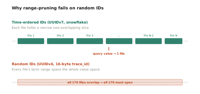
Figure 1 · Range-pruning works only when value ranges don't overlap. Random IDs guarantee they do.

This is the cost we measured. 170 files × one S3-class fetch per file ≈ 2.6 seconds, even with footer cache, even with the right compact size. The footer cache, the compact size — those tools just don't reach this regime.

You can feel the shape of the new tool we need. Something that says "this value is not in this file" before tantivy is allowed to open anything. Cheap enough to be free. Wrong sometimes, but never wrong in the dangerous direction.

That's a bloom filter. The interesting part isn't that; it's where you put it.

The naive bloom filter doesn't work

The most obvious place to put a bloom is one bloom per file. Each parquet gets a sidecar .bf; the query checks each file's sidecar before deciding to open it.

Let's count S3 requests:

• 170 files → 170 sidecar fetches (one GET each)
• Bloom says "maybe" for ~1 file (the real match) and "definitely not" for ~169
• tantivy then opens the 1 survivor

Total: 170 + 1 = 171 S3 requests. Versus tantivy alone at 170. The naive bloom is a tie at best, a loss after constants.

And it's worse than that. Each per-file bloom must be sized for that file's cardinality — for a stream with 10 million unique trace_ids per hour spread across 170 files, each bloom is ~2 MB. The blooms themselves are now the bottleneck.

The problem is the geometry. A bloom filter is fundamentally a "look up a few specific bits in a fixed bit-vector." When you have 170 of them, you're doing 170 small reads — exactly the round-trip pattern S3 punishes hardest.

So the question becomes: can we lay out 170 blooms so that one query value touches only one read across all of them?

The transpose

The bloom filter format used here is the Split-Block Bloom Filter (SBBF) — the same shape Parquet uses internally. An SBBF is a flat array of 32-byte blocks. To check membership for a value:

1. Hash the value to a 64-bit number.
2. Compute block_index = fastmap(hash, num_blocks) — picks one 32-byte block out of the array.
3. Read that block, run a fixed set of bit checks.

The key observation: if every file's bloom uses the same num_blocks, then a given query value maps to the same block index across every file's bloom. Block 7 in file A and block 7 in file B are both "the block that holds membership info for hash %ⁿ = 7."

Now flip the storage layout. Instead of laying out the bytes file-by-file:

file 1: [block 0][block 1][block 2]…[block B-1]
file 2: [block 0][block 1][block 2]…[block B-1]
file 3: …

Lay them out block-by-block:

block 0: [file 1][file 2][file 3]…[file 170]
block 1: [file 1][file 2][file 3]…[file 170]
block 2: …

Now block 7 for all 170 files is one contiguous 5,440-byte row on disk. A single GetRange request fetches it. Inside the response, file 1's block is bytes 0–32, file 2's is 32–64, and so on. One read, 170 membership checks.

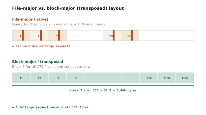
Figure 2 · The transpose turns 170 small reads into 1 contiguous read. Same total bytes; ~170× fewer round trips.

That's the trick. Same total bytes on disk. Roughly the same membership cost. ~170× fewer S3 round trips.

The numbers

The experiment: same stream benchtest, 170 files, 14.64 GB of tantivy index, single matching row, no disk cache, S3 backend. Two fields, one random and one time-ordered, queried with equality:

The transposed read cost was exactly what the math predicted. The full 170-file group was answered by one row read of 5,440 bytes (170 × 32) plus a small cached footer. Total bloom-related network traffic for the whole run: ≈ 170 KB across ~30 requests, almost all of it footer warmup that subsequent queries reuse.

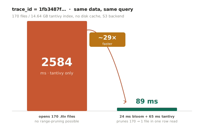
Figure 3 · The random trace_id case. Bar heights are drawn to the real 29:1 ratio.

The transposed layout collapses a whole hour of files into one row read of 5,440 bytes.

The result that surprises people

Look at the second row of that table again. request_id — a UUIDv7, structurally identical to trace_id except for one detail. Its first 48 bits are a millisecond timestamp.

That single detail makes UUIDv7 time-ordered. Files written sequentially carry non-overlapping ranges of request_id values. Tantivy's sparse index range-prunes 169 of 170 files from memory with zero S3 IO. It answers the query in 154 ms.

Add bloom filter pruning on top, and the query gets slower. The bloom layer pays 42 ms to look up a value across a group. Tantivy still takes the same 154 ms on the one survivor (bloom can't tell tantivy to skip the actual matching file). Total: 196 ms. Bloom is pure overhead.

Same code, same data, same query shape. The only variable is whether the values are time-correlated. UUIDv4 wins by 29×. UUIDv7 loses by 1.3×.

⚠️ Why this matters operationally

The choice between UUIDv4 and UUIDv7 is often made by whoever set up the upstream service, for reasons completely unrelated to query performance. They both look like 16-byte UUIDs. Their query characteristics are diametric opposites.

This is why the bloom filter layer in OpenObserve does not auto-detect which fields to bloom. The operator opts in per-field, because the operator knows their ID scheme. Auto-detection from sampled values would be wrong about half the time.

The three conditions for enabling bloom

Bloom is one of those features where "should I turn it on" has a real, principled answer rather than a vibes-based one. Enable it when, and only when, all three of these hold:

1. High cardinality. The field has many distinct values. Otherwise tantivy is already cheap and the bloom is wasted bits.
2. Random, not time-ordered. The value distribution does not correlate with insertion time, so tantivy's sparse index cannot range-prune and is forced to open every .ttv. This is the wedge bloom exploits.
3. Many files per hour. Bloom's whole job is "turn N file opens into one row read." If the hour has 1 or 2 files there is nothing to prune and the row read is net overhead. As a rule: enable when hourly volume is at least ~10× ZO_COMPACT_MAX_FILE_SIZE.

The summary table for the operator:

Worth being explicit about one constraint: bloom is built on top of tantivy, not alongside it. The .bf is constructed by iterating the tantivy term dictionary at compaction time. So a field has to be in both index_fields (the tantivy secondary index list) and bloom_filter_fields for a bloom to be built. The intersection is what gets covered. A field in only bloom_filter_fields has no term dict to read and silently produces no bloom.

The design details that matter

A few things from the implementation that are worth pulling out, since they shape the cost model.

The .bf file format

One .bf per (stream, hour, chunk). A chunk caps at ZO_BLOOM_FILTER_MAX_FILES_PER_BF files (default 256) so the writer's memory usage stays bounded. An hour with more than 256 files produces multiple .bfs; the query reads one row per .bf, so query cost grows as ceil(files / 256) reads — still O(1) per hour for typical scales, and the read sizes stay small (≤ 256 × 32 = 8 KB).

The footer holds field metadata and per-file (file_id, n_items) tuples. It's typically ~12 bytes per file, so well under 16 KB for a 256-file .bf. A small in-memory footer cache (mirroring the tantivy footer cache from the previous post) means a warm bloom lookup is one row read; a cold lookup is one suffix probe plus one row read.

Performance, not correctness

Every failure mode in the bloom layer degrades to "keep the file." A .bf fetch that times out, a parse error from a corrupt blob, a schema-drifted field that's missing from a particular file, a file whose bloom_ver is still zero because the bloom build hasn't run yet — all of these collapse to "let the file fall through to tantivy." The original search path is still there underneath. The bloom layer is allowed to silently fail; it is never allowed to silently drop a row.

Operationally this matters because it means bloom can be enabled with no risk of incorrect query results. The worst it can do is be slow.

What changes for users

Two settings, plus the per-stream field list:

ZO_BLOOM_FILTER_ENABLED = true            # global gate
ZO_BLOOM_FILTER_MAX_FILES_PER_BF = 256    # chunk size knob

And on each stream where bloom should apply:

index_fields:        ["trace_id", "request_id", ...]
bloom_filter_fields: ["trace_id"]   # subset that's random + high-cardinality

The intersection of these two lists is what gets a bloom. Pick fields where all three conditions hold. When in doubt, leave it off — the cost of having bloom off for a field that could benefit is at most "as slow as before," but the cost of having it on for a field that doesn't benefit is real overhead on every query.

And, related to the previous post: keep the compact file size at 10 GB (ZO_COMPACT_MAX_FILE_SIZE = 10240). The same logic compounds. Fewer, larger files mean fewer hourly buckets, fewer .bf reads, and less work per query at every layer of the stack.

Worth flagging: bloom filter is a new feature for performance optimization, will be released in the next version.

The bottom line

The previous post collapsed S3 request count for the common case. This post handles the case the previous one couldn't:

For random high-cardinality lookups, OpenObserve can now answer a query against 170 files of tantivy index with one row read of 5,440 bytes.

The win is mechanically the same kind as the previous one — cutting S3 round trips by an order of magnitude — but the lever is different. There, it was compacting more aggressively and caching footers. Here, it's a transposed bloom filter layer that takes a problem tantivy can't help with and answers it before tantivy is even asked.

What this looks like end to end:

• If your stream has high-cardinality time-ordered IDs only, you already won. Tantivy's sparse index handles you for free; do nothing.
• If your stream has high-cardinality random IDs that you query by equality often (and most observability streams do — trace_id is the canonical one), enable bloom on those fields. Expect order-of-magnitude improvements on lookup queries.
• If you're unsure which category your IDs fall into, look at how the upstream service generates them. UUIDv7 / snowflake / timestamp-prefixed = time-ordered. UUIDv4 / random hex / hashed = random.

It's a layer that's invisible when it shouldn't help, and large when it should.

The query that used to take 2.6 seconds now returns in 89 milliseconds.

Test notes:

• All numbers from a single querier on S3-backed storage with no disk cache, against the benchtest stream (170 parquet files / 14.64 GB tantivy index for the hour under test)
• "29×" is rounded; raw ratio is 2584 / 89 ≈ 29.04
• The bloom layer ships behind ZO_BLOOM_FILTER_ENABLED; enable per-stream by adding fields to bloom_filter_fields (must also be in index_fields)
• The transposed layout caps each .bf at 256 files by default (ZO_BLOOM_FILTER_MAX_FILES_PER_BF); larger files-per-hour split into multiple .bfs with one row read each
• Bloom build adds storage cost proportional to total cardinality (~10 bits per unique value at 1% FPR); a 10M-unique-value field across 256 files ≈ 4 GB per .bf. Budget this before enabling on extreme-volume streams

Take the Next Step

New to OpenObserve? Register for our Getting Started Workshop for a quick walkthrough.

• Download OpenObserve for self-hosting
• Sign up for OpenObserve Cloud — 14-day free trial, no credit card required