OpenObserve vs ClickHouse: One Billion Log Records

TLDR

• We generated one billion log records, 2,199 GB of raw NDJSON, serialized each record once, and wrote the identical bytes into ClickHouse and two OpenObserve instances at the same time, each on its own dedicated node. Then we stopped ingestion and ran the same 19 queries against each, one backend at a time. Everything is in the benchmark repository.
• OpenObserve answers a typical query 2.7x (Parquet) to 3.4x (Vortex) faster than ClickHouse, by geometric mean across the 19 queries, and finishes the whole suite in 3.4x to 4.6x less total time, on a third less disk, with a full-text index on both sides.
• The gap is not uniform. ClickHouse wins two of the 19 outright, both small: the newest 100 rows on a common term, where its _timestamp sort key lets it read the tail of the table and stop, and a two-term intersection. It ties two more at the millisecond floor. On the other ID and term lookups OpenObserve is 1.1x to 5x faster on Parquet and 1.4x to 6x on Vortex, and on the three queries that have to touch most of the billion rows, a high-cardinality count, a common-token count, and an hourly histogram, it is 25x to 109x slower.
• One setting was worth more than the file format. Raising OpenObserve's compaction target file size from its 2 GB default to 10 GB was a 2.1x to 2.3x geometric-mean improvement, and it is what moves the per-query advantage over ClickHouse from 1.3x to 1.4x up to 2.7x to 3.4x. The one regression, Parquet row fetch by a high-cardinality column, went 2.0x slower; Vortex did not, and Vortex is 2.6x faster than Parquet on row fetches overall.

Why compare OpenObserve and ClickHouse for logs

Every generation of log storage has been a general-purpose tool pointed at logs. Lucene was a text search library; Elasticsearch wrapped it and became the log store of the 2010s, until the memory and the operational weight of running a search engine as a database stopped being worth it at scale. Columnar OLAP is the next generation, and ClickHouse is its best-known engine: fast, mature, and the engine under a lot of serious logging stacks. It is a much better fit than Elasticsearch was.

It is still a general-purpose engine, and that is the question this benchmark asks. A system that serves every analytical workload has to leave the choices to you: the sort key, the index types, the schema, the product around it. Each choice is a trade, and a trade that is right for one query shape is wrong for another. A system built for one workload can make those choices once, and can add structures that make no sense for a general database, because "find every line from this pod" is its whole job rather than an edge case. Whether that is worth anything is an empirical question, so we measured it.

The two systems get there differently. ClickHouse is a general-purpose analytical database: you design the schema, choose the sort key, choose the skip indexes, and build collection, dashboards, and alerting around it. OpenObserve is a single Rust binary that is the whole observability stack, logs, metrics, traces, dashboards, alerts, RUM, synthetics, and SLOs, with schema inference on ingest and object storage as the durable layer. Both store data in columnar files. ClickHouse writes MergeTree parts to local disk; OpenObserve writes Parquet or Vortex, both open formats that Spark, DuckDB, and Pandas can read directly.

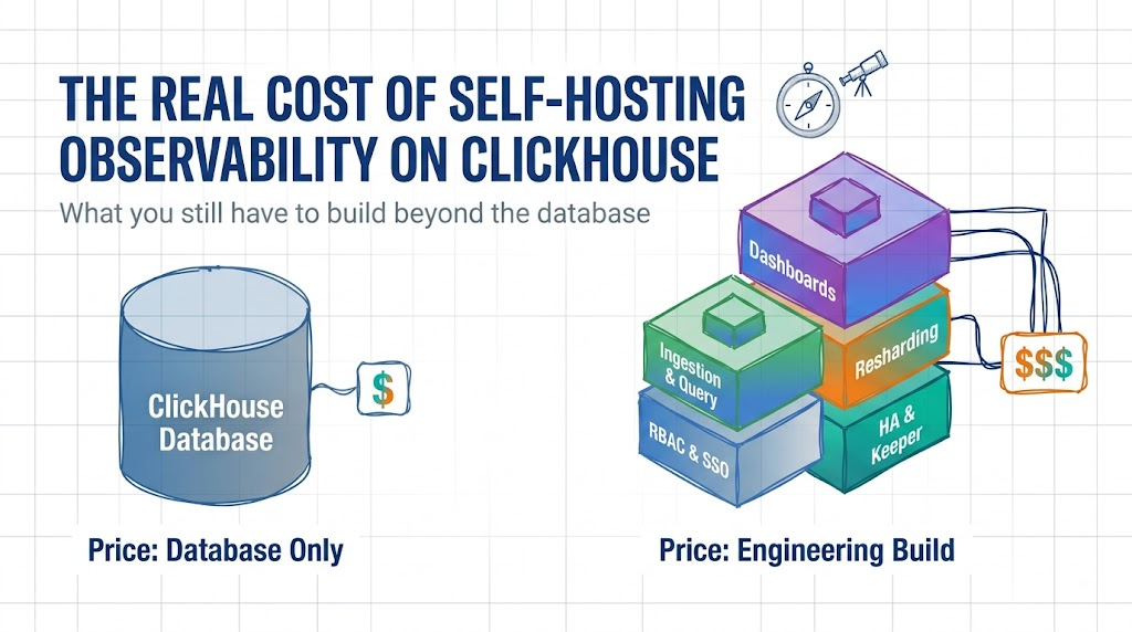
We have compared the two before, on a smaller and differently shaped run, in OpenObserve vs ClickHouse: which is better for logs and on the economics in the cost of self-hosting observability on ClickHouse. This run is a rebuild of the query benchmark at a billion records with much tighter controls, and it produced a result we did not expect, which is most of why it is worth reading.

How we ran it

The methodology decides a benchmark like this more than any single number, so here it is in full. The generator, the schemas, the query templates, the runner, and every raw sample are in the benchmark repository.

Hardware and versions

Three single-node deployments, one per dedicated EC2 i8g.2xlarge with data on that node's local NVMe. The nodes run concurrently and share no hardware, so CPU, memory, disk bandwidth, and page cache are never contended between engines. Only the measurement is serialized, one backend at a time, so no engine is answering queries while another is being timed.

• ClickHouse 26.7.3.19-stable, MergeTree ORDER BY (_timestamp)
• OpenObserve v0.92.2 with ZO_FILE_FORMAT=parquet
• The same OpenObserve binary with ZO_FILE_FORMAT=vortex

A fourth node, a c7g.2xlarge not under test, runs the data generator and the benchmark client.

The dataset

1,000,000,000 records, 2,199 GB of raw NDJSON, 27 columns of Kubernetes-shaped log lines spanning about 4h13m of event time.

Ingestion is a single fan-out pass: the Rust generator serializes each record once and posts the same bytes to /_multi on both OpenObserve instances and JSONEachRow on ClickHouse. A batch counts as sent only when every backend accepted it. That took 16,666 seconds (4h37m) of wall clock at 60,002 rec/s and 128.1 MB/s, and then it stopped. Three independently generated datasets would not be comparable, so there is only one.

The queries

19 queries, each expressed natively per engine over an identical, absolutely pinned time window:

• 8 indexed count() queries
• 3 full-scan aggregations
• 8 SELECT * … ORDER BY _timestamp DESC LIMIT 100 row fetches

Each runs 5 times. The OS page cache is dropped on the backend node itself (sync; echo 3 > /proc/sys/vm/drop_caches) immediately before that backend's pass, so run 1 is cold and hot is min(run 2, run 3), the convention the repository's interactive report uses; all five runs are in the repository. The dataset is 674 GB to 1 TB against 64 GiB of RAM, so the cache can hold only a small fraction of it in any case.

Index parity is the hard part

A log benchmark is decided by its indexes, so both engines get the same ones:

kubernetes_container_name is left unindexed on purpose. It has 8 distinct values, so each one matches about an eighth of the dataset and appears in nearly every file: a bloom filter rejects no granules and a secondary index returns a posting list too large to be worth merging. Four of the 19 queries filter on it, and giving the index to one engine and not the other would make those four results measure the setup rather than the engine. Parquet's embedded row-group bloom filter is disabled (ZO_BLOOM_FILTER_PARQUET_ENABLED=false) so it cannot become a Parquet-only advantage over Vortex. ClickHouse is ordered by _timestamp alone, so no structured column gets a sort-key advantage either.

How much tuning is this

We kept the effort symmetric across both the engines. ClickHouse got one straightforward schema with matched indexes and no further work. OpenObserve got its defaults and, in round 2, one setting. We show both rounds so the effect of that one line is visible rather than baked in. Both engines have more headroom than this, and on both sides it comes with trades. A ClickHouse engineer would start with a pod-first sort key and column codecs: the sort key would take the 109x pod_name count off the board and likely flip the pod_name row fetch, and it would cost ClickHouse the newest-rows-on-a-common-term query it currently wins, because that win depends on _timestamp being the only key. An OpenObserve engineer would start with the compaction target, which is why it is in the post, along with the one query it made slower. We think this level of effort is closer to what a team evaluating the two would actually run than a specialist-tuned shootout, and the repository is there for anyone who wants to run that one.

Fairness controls

• Query caches off on both sides. ClickHouse runs with enable_filesystem_cache=0; OpenObserve with use_cache=false as a URL parameter, which is the only place that flag is honoured.
• Nothing under test also drives the test. A driver co-resident with a backend would burn CPU on JSON serialization and result parsing on the very box it is timing, and would do so unequally across three engines that return different payload sizes. Keeping it on a fourth node costs one instance and removes the whole class of problem.
• Both sides report their own time. ClickHouse's statistics.elapsed and OpenObserve's took are both server-side, so neither engine is charged for HTTP or client overhead the other avoids, and the network hop between driver and backend is not charged to either. That only works because the driver is off the measured nodes; the two choices go together.
• Read millisecond ties as ties. OpenObserve reports took in whole milliseconds. Below about 30 ms that quantization is a real part of the spread, and a two or three millisecond gap in the tables below is a tie, not a win.
• No projections or materialized views on either side. Both are precomputed answers to queries you already know you will run, and this is a benchmark of raw engine performance: what each engine does with a query it has not seen, over data it has only indexed. ClickHouse's sort key, skip indexes and text index are all in play, and so are OpenObserve's Tantivy full-text and secondary indexes. Nothing that amounts to caching the answer is.

And the disclosure that belongs in every vendor benchmark: we make OpenObserve. The repository exists so you can rerun everything on your own account and tell us where we are wrong.

What this benchmark does not measure

• Ingestion throughput per engine. The 16,666-second figure is one fan-out pass feeding all three backends at once, gated by the slowest of them plus the generator. It is a statement that all three received identical data, not three ingest results.
• Time-range pruning. The query window is a full year wrapped around a 4h13m dataset, so every query touches all of it. That is identical for both engines and the worst case for both, but nothing here rewards partition pruning.
• Concurrency. Every query is issued serially against an otherwise idle machine.
• Per-query row counts. The harness reads rows_read (ClickHouse) and scan_records (OpenObserve) on every request but does not persist them, so the recorded results carry latency without the work behind it. The row check that is recorded sits at storage level, system.parts against file_list, and confirms all three backends hold the same 1,000,000,000 rows. Persisting the per-query counts is the first thing to add before the next run.

Storage

Taken from each engine's own metastore: system.parts plus system.data_skipping_indices for ClickHouse, the stream-stats API backed by file_list for OpenObserve. Both figures are compressed data plus indexes, measured at the round-1 setting.

OpenObserve stores the same billion records in a third less space than ClickHouse, while carrying a Tantivy full-text index that ClickHouse's text() index is the counterpart to. Raising the compaction target to 10 GB grew both OpenObserve footprints by 0.49 percent, since larger merge units produce marginally larger output. That is noise next to what it does to query latency.

Round 1: stock configuration

This suite total favors OpenObserve:

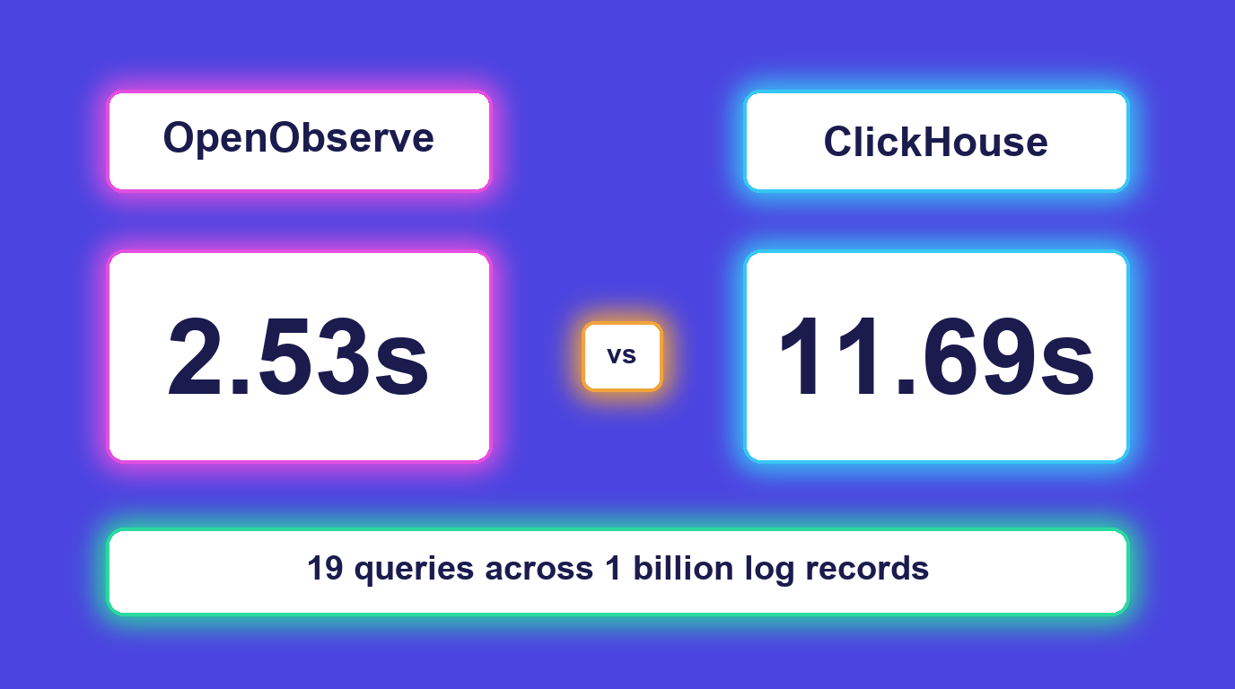
11,578 ms for ClickHouse against 4,663 ms for Parquet and 4,106 ms for Vortex.

That total is concentrated in four queries where ClickHouse has to read most of the billion rows: the pod_name count, where its bloom filter rejects almost no granules for a pod present everywhere; the common-token count, where the text index finds the term everywhere and then counts; and the two histograms, which are full scans by design. OpenObserve answers the first two out of its index. Remove those four, the four widest gaps in the suite, and the remaining 15 are roughly even:

Per query, OpenObserve wins 10 of 19 on Vortex and 9 of 19 on Parquet, and ClickHouse takes most of the single-index lookups, because at this setting every OpenObserve lookup pays a fixed 96 to 100 ms before it starts. Round 1 is a win on the four widest-gap queries, and ClickHouse takes most of the small ones by the width of that fixed per-file cost, which is what round 2 removes.

Buried in the round-1 numbers is the most informative result in the whole benchmark, a number that refuses to vary:

Six queries with completely different selectivity, hitting three different index types: a bloom-backed ID lookup, a full-text term that matches almost nothing, a full-text term that matches a large fraction of the dataset, and a secondary index on a high-cardinality column. They all answer in 96 to 100 ms.

That is not six query costs. It is one fixed cost, paid before any of them start, with the actual query work disappearing underneath it.

Round 2: one knob, ZO_COMPACT_MAX_FILE_SIZE=10240

Same dataset, same queries, same machines. OpenObserve's compaction target file size raised from its 2 GB default to 10 GB, which is roughly a fifth as many data files, each five times larger. ClickHouse was left untouched and re-measured, which makes it the control.

The control first

That is the run-to-run noise floor of the whole harness. Every OpenObserve change below sits far outside it.

The floor collapses

The six queries pinned at 96 to 100 ms land at 24 to 28 ms, a 3.8x drop that is close to the roughly 5x reduction in file count. That is the signature of a per-file fixed cost: opening files, reading their metadata, loading their index segments, merging their results. It scales with how many files a query touches, not with how much data it reads, which is exactly why it was identical across six queries doing entirely different work. Fewer, larger files pay it fewer times.

It also explains the shape of the rest of the suite. Queries already dominated by real work barely move: top-N namespaces, a full scan and group-by over a billion rows where per-file overhead is a rounding error, improves only 1.07x on Parquet and 1.14x on Vortex.

Hot, ms. Δ is round 1 divided by round 2, so above 1.00x is faster after the change. Bold marks a change of 1.3x or more in either direction.

The one that got slower

Fetching 100 rows by kubernetes_pod_name got 2.0x slower on Parquet: 321 ms to 654 ms hot, and 395 ms to 857 ms cold. It is the only regression in 38 measurements, and it is worth being precise about what the data actually supports:

• It is Parquet-specific. The same query, on the same data, with the same 10 GB cap, got faster on Vortex, 114 ms to 103 ms. So the cause sits in the read path, not in compaction itself.
• It is row-fetch-specific. The pod_name count() query uses the same secondary index over the same rows and improved 3.70x. Only materializing the rows regressed.
• It shows up cold and hot alike, at a similar ratio, so it is not a cache artifact.

The likely mechanism, and this is a hypothesis rather than something this run profiled, is that a top-K row fetch has to materialize candidate rows out of whichever files the index points at, and a 10 GB Parquet file makes that unit of work five times larger: a footer five times bigger to deserialize, five times the row groups to seek through, larger column chunks to decompress, all to return 100 rows. Vortex's layout is lazily addressable, so the same lookup does not pay in proportion to file size.

The practical reading: if your workload is dominated by SELECT * … LIMIT n on a secondary-indexed high-cardinality column and you run Parquet, measure before raising this knob. On Vortex it is a straight win.

Round 2: head to head

Hot, in milliseconds, all three systems at their round-2 settings. The 19 queries are numbered Q1 to Q19 in the order they appear here, and the rest of the post refers to them by number. Bold is the fastest in the row, and every cell within 3 ms of it where the fastest is under 30 ms, per the tie rule above. The wins / ties / losses counts further down apply the same rule against ClickHouse specifically.

Indexed count()

Full-scan aggregation

SELECT * … ORDER BY _timestamp DESC LIMIT 100

Aggregate

The geometric mean is the number to quote for "how much faster is a typical query," because it is not swayed by which queries happen to be slowest. The total is the number for "how long does this whole batch take," and it is dominated by the four queries with the widest gaps. Both are in the table; the geometric mean comes first because most log queries are issued one at a time by a person who is waiting.

ClickHouse is outright fastest on 2 of the 19 and tied on two more at the millisecond resolution floor. The compaction change takes OpenObserve to 14 wins on Parquet and 15 on Vortex, with the geometric-mean advantage going from 1.26x to 2.74x on Parquet and from 1.44x to 3.35x on Vortex. The same slice test as round 1 now holds at every cut:

Parquet's margin on the last row is thin because of one query, the pod_name row fetch (Q19) at 654 ms, covered above. Remove that as well and Parquet is 1.33x on the remaining 14.

By query class

Indexed counts are a 22x to 24x win on the class total: 3x to 5x on the ID and compound lookups, two ties at the floor, one loss on the two-token intersection, and two very large wins where ClickHouse's index cannot produce a count without reading the table. Aggregations are 2.5x to 2.9x on the class total. Row fetch is where the two formats part: Vortex is 2.4x faster than ClickHouse on the class total and wins 7 of 8. Parquet wins 6 of 8; its class total, 1,114 ms against 1,038, is carried entirely by the 654 ms pod_name fetch (Q19), and on the other seven it is 460 ms against 843.

Where the gap is widest

kubernetes_pod_name has a bloom_filter(0.01) skip index on the ClickHouse side and it still takes 2.9 seconds, because a bloom filter can only reject granules, and for a pod that appears throughout a billion rows very few granules can be rejected. OpenObserve's Tantivy secondary index returns the matching row set directly. The same asymmetry drives the common-token count: ClickHouse's text() index finds the term everywhere and then counts, while OpenObserve reads the count out of the index.

The hourly histogram is the same kind of win, and it is worth being plain that it is not a scan either. OpenObserve's planner recognises the shape, GROUP BY histogram(_timestamp) with only a count(*) and no other predicate, and answers it from the index files without opening the Parquet or Vortex data at all, which is why the two formats tie at exactly 63 ms. Each index file stores _timestamp as a sorted column, so the count in a bucket is the difference between two binary searches for the bucket edges: a handful of probes per file, not a visit to any row. ClickHouse has no equivalent shortcut, because its primary index is sparse, one mark per 8,192-row granule, so it can prune granules but cannot count rows between two arbitrary timestamps without reading them, and toStartOfHour plus a hash GROUP BY over a billion timestamps is what 1.6 seconds buys. Two caveats. The shortcut is specific to that query shape: add a second aggregate such as avg(http_latency_ms) and the query goes back to a full columnar scan. And top-N namespaces (Q10), at 1,639 ms against 1,500 and 1,204, is the one query in this suite where both engines genuinely scan a billion rows, so it is the honest measure of scan speed; the 25x on the histogram is an index-structure win, not a scan-speed win.

Every row ClickHouse ties or wins

Only two of those are outright ClickHouse wins over both formats. Two are ties at the floor, and Vortex takes the pod_name row fetch. There is a clear pattern: ClickHouse wins where its ORDER BY (_timestamp) sort key lets it answer a top-K query by reading the tail of the table, and where intersecting two text terms lets the text index do almost all the work. It loses by 25x, 70x, and 109x on the three queries that have to touch most of the table: the hourly histogram (Q9), the common-token count (Q4), and the high-cardinality pod_name count (Q8).

Parquet vs Vortex

The two OpenObserve instances share a binary, a dataset, an index configuration, and every environment variable except ZO_FILE_FORMAT.

They are level on indexed count(), because both are answering out of the same Tantivy index and the format barely participates. The gap is entirely in the two groups that read data:

• Row fetch: Vortex is 2.6x faster in aggregate, and wins all eight individually. Materializing 100 wide rows out of a large file is exactly what its lazily addressable layout is for, and it is also why Vortex did not regress where Parquet lost 2x on pod_name row fetch.
• Aggregation: Vortex leads by 1.16x, almost all of it from top-N namespaces at 1,204 ms against 1,500 ms.
• Storage: Parquet is 5.2 percent smaller.

For a log-search workload, find the matching lines and show me the lines, Vortex is the better default, and the storage difference is not close to paying for it.

Where ClickHouse wins

An honest benchmark reports its losses, and ClickHouse takes real ones here.

• Selective top-K queries on the sort key. ORDER BY (_timestamp) lets ClickHouse answer "newest 100 rows matching a common term" by reading the tail of the table and stopping. It does that in 26 ms against OpenObserve's 47 to 52 ms.
• Intersecting two text terms. A common AND rare token count is 25 ms on ClickHouse against 41 and 45 ms. Intersecting two posting lists is cheap and it does it well.

Where OpenObserve wins

• The queries that have to touch most of the table. 109x on a high-cardinality pod count, 70x on a common-token count, 25x on an hourly histogram over a billion rows. These are the shapes typical of log dashboard panels.
• Typical and total latency across a realistic suite. 2.7x to 3.4x per query by geometric mean, 3.4x to 4.6x on total suite time, and faster on 14 or 15 of 19 individual queries.
• Disk. A third less than ClickHouse for the same billion records, with a full-text index included in the number.
• Open formats, no proprietary storage. Parquet is an Apache standard and Vortex is a Linux Foundation project, so Spark, DuckDB, and Pandas read the files directly.
• An observability data lake. Data lands in open formats on object storage, which makes your telemetry an owned, queryable asset rather than rows inside one engine.
• A complete platform in one binary. Logs, metrics, traces, dashboards, alerts, RUM, synthetics, and SLOs. Building the same thing on ClickHouse means assembling collection, schema management, dashboards, and alerting around it yourself.

What the benchmark held constant

Every number above was measured with all three systems on local NVMe, because the benchmark is about the engines and storage was deliberately not a variable. Two things that are constant in the benchmark are not constant in production, and both favour OpenObserve by more than any query result.

Where the data lives. OpenObserve is object-storage native: the durable copy of every file is in S3 (or GCS, Azure Blob, MinIO), and local NVMe holds only a cache. ClickHouse does support S3 as a disk, and a reader who knows that will object here, so the distinction matters. Open-source ClickHouse can put MergeTree parts on an S3-backed disk, but MergeTree was built around local storage: S3-backed parts are slower to query, merges rewrite data through the object API, and every replica still owns its own copy. The engine that genuinely separates compute from storage, where replicas share one copy in object storage and local disk is only a cache, is SharedMergeTree, and SharedMergeTree is proprietary to ClickHouse Cloud. It is not available to a self-hosted deployment at any price. So a self-hosted ClickHouse keeps its working data on attached disk, and high availability means two or three replicas each holding a full copy.

The arithmetic at list prices: EC2 instance-store NVMe works out to roughly $0.14 per GB-month; S3 Standard is $0.023. Two replicas on NVMe is about 12x the per-GB cost of a single copy in S3, three replicas about 19x, before S3 request costs and before the NVMe cache OpenObserve keeps in front of it. Combined with the 0.66x to 0.69x on-disk footprint measured above, the durable-storage bill for the same billion records is an order of magnitude apart. The full cost model, including compute and operations, is in the cost of self-hosting observability on ClickHouse.

How it scales. Because the data is in the bucket, OpenObserve's ingesters, queriers and compactors are stateless: scaling out is adding nodes in front of the same object store, and a node that dies loses nothing. Self-hosted ClickHouse scales by shards and replicas coordinated through Keeper, each replica owning its data, so growth means resharding a stateful cluster, and adding replicas multiplies the disk bill above. The stateless model exists for ClickHouse too, and it is the same answer: SharedMergeTree, in ClickHouse Cloud only. Neither of these shows up in a single-node benchmark. Both show up in the second year.

What to take away

Tune the file size before you tune the format. The most useful result in this benchmark for anyone running OpenObserve is not the ClickHouse comparison, it is what one setting did to OpenObserve itself. One compaction setting was worth 2.1x to 2.3x geometric mean, more than the difference between Parquet and Vortex on most of the suite, and it is the difference between a 1.3x to 1.4x per-query advantage over ClickHouse and a 2.7x to 3.4x one. If you run OpenObserve on logs at this scale, ZO_COMPACT_MAX_FILE_SIZE is the first thing to look at.

Two caveats on that. It is a compaction-time setting, so it changes the files compaction produces and does nothing to files that already exist: set it before ingesting, or force a recompaction pass over existing data and wait for it to finish. And on Parquet it has one sharp edge, the 2x regression on SELECT * … LIMIT n by a high-cardinality column, which Vortex does not have.

Then pick Vortex. For log search it is faster where it counts, 2.6x on row fetch, and it is the format that did not regress.

On ClickHouse. If your log queries are almost all newest-N-by-time on a term that matches most rows, ClickHouse wins that shape and this benchmark says so. If they include dashboards, histograms, group-bys, or counting anything across a high-cardinality dimension, which is the usual shape of log analytics, the gap on the heaviest of them is one to two orders of magnitude, and it is the gap between a panel that loads and a panel you stop opening.

That is the general-tool cost in one table: ORDER BY (_timestamp) is the right choice for top-K-by-time and the wrong one for everything that filters on a high-cardinality column, and a general-purpose engine cannot make that choice for you.

Check it yourself

Nothing here is a screenshot of a number we ask you to trust. The entire benchmark, data generator, ClickHouse schema and index definitions, the matched query templates for both engines, the isolated runner, the report builder, and the raw per-run samples behind every figure in this post, is in one public repository:

github.com/openobserve/openobserve-clickhouse-benchmark

That includes the parts that make a benchmark arguable rather than merely quotable: which columns are indexed on each side and why, the exact SQL each engine was asked to run, and all five raw samples for every query, engine, and round. Any table here can be recomputed, and any choice we made can be changed and rerun.

Two things to watch if you do. The page-cache drop has to happen on the backend node, not on the driver, or you are measuring a warm cache and the harness will still report success. And verify the row counts match on all three backends before measuring anything, after waiting for compaction to finish.

If you reproduce it and get a different answer, that is a useful result. Open an issue with your numbers.

Try OpenObserve

If a log store that answers a high-cardinality count in 27 ms at a billion records on a third less disk sounds useful, the fastest way to feel the difference is to point some real logs at it. OpenObserve Cloud gives you ingestion, full-text search, SQL, dashboards, and alerting without running the binary yourself, and the same engine is open source if you prefer to self-host.