OpenObserve vs ClickHouse: Which Is Better for Logs?



Don’t forget to share!



Getting Started with OpenObserve
Try OpenObserve Cloud today for more efficient and performant observability.
TLDR
This is not only a database-versus-database verdict. It compares two ways to build a cloud-native observability system: assemble observability capabilities around a high-performance analytical database, or start with an integrated platform designed around object storage. The benchmark addresses the question that remains after cost, architecture, and operations enter the decision: does the integrated approach require giving up query performance?
We wanted a straight, reproducible answer, so we ran OpenObserve and ClickHouse on matched hardware, with the same data and the same queries, at a billion rows, and we ran it twice, on two different disk tiers. OpenObserve can run as a single Rust binary and stores logs, metrics, and traces as Parquet, with object storage as the durable data layer in its cloud-native architecture. ClickHouse is a column-oriented analytical database that many teams, and products such as SigNoz and ClickStack, use as an observability store.
ClickHouse earned its place in observability honestly. ClickHouse Inc.'s internal logging platform stores 431 PiB of uncompressed telemetry across 1.59 quadrillion rows, compressed to 27 PiB on disk (ClickHouse blog, June 2026), and companies like Last9 push 480 million log lines per minute through it (ClickHouse blog, April 2025). As a column store with strong compression, it is a good place to keep log data.
The difference is what surrounds the store. Bare ClickHouse gives you a fast engine and SQL; you design the schema, indexes, ingestion and retention policies, and add an observability-specific query service and UI. Products such as SigNoz and ClickStack package those surrounding layers. OpenObserve takes the other path: it integrates ingestion, indexing, retention, search, dashboards, and alerting in one product, with defaults tuned for logs. Its single-node mode can run as one binary; its HA architecture adds the infrastructure required for durability and scale while keeping the observability experience integrated. If you are weighing self-hostable options, this is the same decision you face when you read our roundup of open source observability tools or compare Elasticsearch alternatives, where ClickHouse also comes up as a logs backend.
Cost keeps this comparison honest. In Grafana's 2025 observability survey, 74 percent of respondents said cost is a top factor when picking observability tools, and the average organization runs eight observability technologies (Grafana 2025 survey). Log volume is the reason: Chronosphere's 2024 practitioner survey found log data growing 250 percent year over year on average (Chronosphere, October 2024). Storage and query efficiency are not academic here. They are the bill.
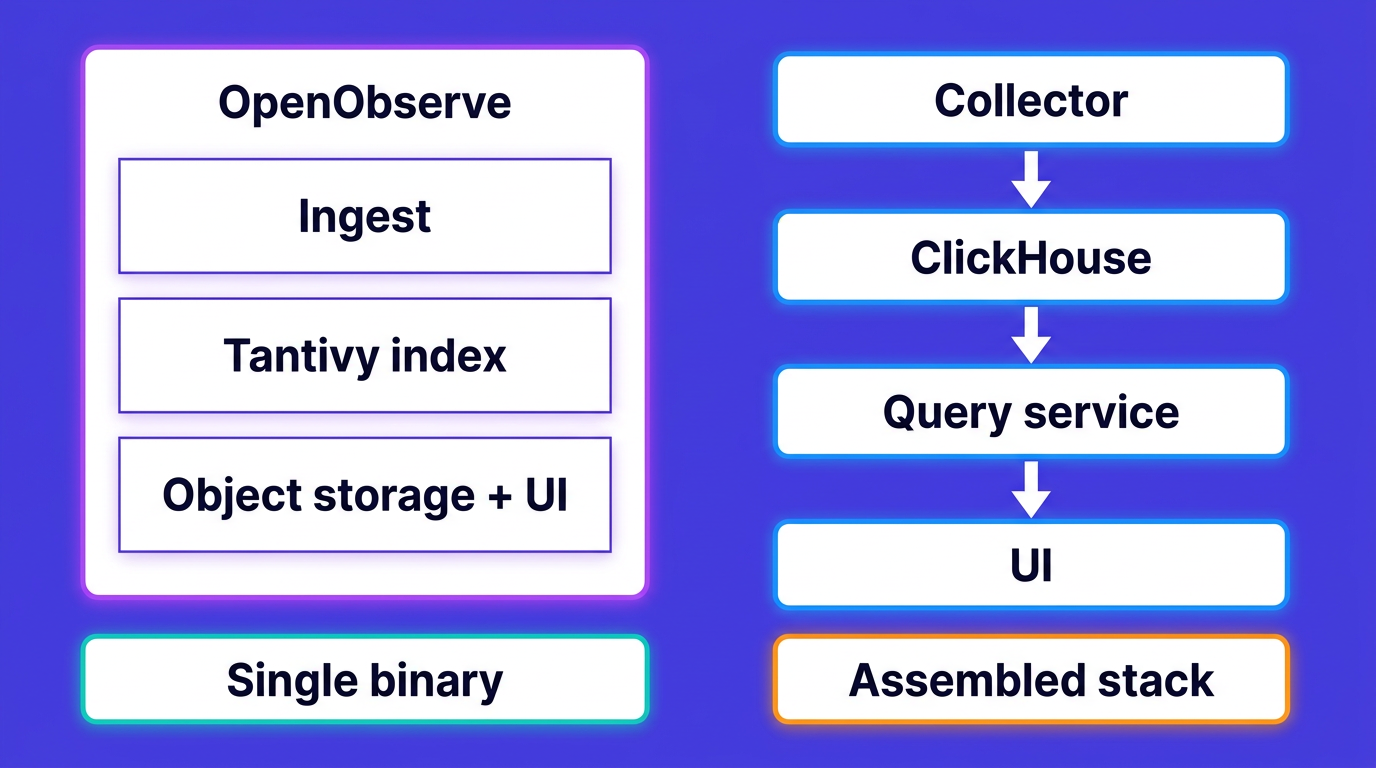
The diagram compares the observability application layers supplied by each approach. Both still need a collector for Kubernetes logs, and production HA deployments need supporting infrastructure.
The methodology matters more than any single number, so here it is in full. The driver, the schemas, and every query live in the benchmark repository, so you can reproduce or dispute anything below.
Each engine had its own node, and we benchmarked them one at a time with the driver running on the engine's node. Neither could contend with the other for CPU or page cache. A third identical node ran the data generator.
c7gd.8xlarge nodes (32-core Graviton3, 61.6 GiB usable RAM, 1900 GB local NVMe instance store), Ubuntu 24.04.c7g.8xlarge nodes, each engine on a 2000 GiB gp3 EBS volume provisioned at 16,000 IOPS and 1000 MB/s, which is gp3 at its maximum throughput, so the comparison is against gp3 at its best rather than a throttled default.Note the ratio: 61.6 GiB of RAM against 937 GiB of ClickHouse data and 621 GiB of OpenObserve data on disk. The working set cannot fit wholly in page cache, and the cold run drops the OS page cache before the query to exercise the storage path. Neither run measures either engine querying from S3.
We generated 1 billion synthetic Kubernetes log records with a deterministic Rust generator (fixed random seed) that streams every batch to both backends simultaneously, so they received an identical 1,000,000,000-row stream. The stream is the generator's 100M-record output ingested ten times; we verified row counts against the expected total after every 100M batch, and both engines finished at exactly 1,000,000,000 records with zero failures. The raw JSON totaled 2.04 TiB. Each record carries realistic fields: pod and container names, namespaces, HTTP method and status, trace and span ids, and a log message built from real-world templates. The needles the queries search for hit real data: the benchmark's trace id matches 60 rows out of the billion, verified directly against ClickHouse after ingest.
We ran three families of queries, each published verbatim in the repository, and measured server-side latency five times per query. The first run comes right after dropping the OS page cache, so run one is cold; the warm number is the fastest of the next two runs, matching how the published report page computes it. We report both.
SELECT * ... ORDER BY _timestamp DESC LIMIT 100, which is what a log viewer actually does.Two systems are only comparable if they answer the same questions the same way, so both engines ran the same generated data, the same needles, and the same five-run cold-then-warm protocol, with each engine's own result cache disabled per request. Every measurement is a real search, not a cached answer.
And one disclosure that belongs in every vendor benchmark: we make OpenObserve. Treat the numbers accordingly: the repository exists so you can rerun everything on your own account and tell us where we are wrong.
The most common way a vendor benchmark goes wrong is tuning your own tool and running the competitor near defaults, so here is exactly what each side ran. Read this section before you read the numbers. Both engines had full search indexes on the same fields; neither side ran unindexed.
OpenObserve indexes are set with environment variables before ingest.
ZO_ENABLE_INVERTED_INDEX=true
ZO_FEATURE_FULLTEXT_EXTRA_FIELDS=message
ZO_FEATURE_INDEX_EXTRA_FIELDS=trace_id,span_id,kubernetes_pod_name
That is the entire index configuration. OpenObserve builds a Tantivy full-text index on message and secondary indexes on the marked columns automatically, described in the full-text search functions docs.
ClickHouse needs the same fields indexed through its own native mechanisms: three bloom_filter skip indexes on the high-cardinality columns, and one full-text text() index on message. These indexes cover the same fields, but their data structures and pruning behavior are not identical.
CREATE TABLE k8s_logs
(
    `_timestamp`          UInt64,
    `message`             String,
    `trace_id`            String,
    `span_id`             String,
    `kubernetes_pod_name` String,
    -- 22 more columns, LowCardinality on repetitive string dimensions
    INDEX idx_trace_id   trace_id            TYPE bloom_filter(0.01) GRANULARITY 1,
    INDEX idx_span_id    span_id             TYPE bloom_filter(0.01) GRANULARITY 1,
    INDEX idx_pod_name   kubernetes_pod_name TYPE bloom_filter(0.01) GRANULARITY 1,
    INDEX idx_message_text message TYPE text(tokenizer = splitByNonAlpha, preprocessor = lower(message))
)
ENGINE = MergeTree
ORDER BY (_timestamp)
SETTINGS index_granularity = 8192;
One gap you should know about: this table carries no explicit compression codecs, so it used ClickHouse's default compression. ClickHouse's own observability guidance recommends ZSTD(1) on columns and Delta plus ZSTD(1) on a monotonic timestamp, which compresses log data considerably better than the default. We did not apply them. That affects the storage numbers below, and to a lesser degree the cold reads, so treat this run as ClickHouse at default compression rather than ClickHouse tuned for storage.
Two more choices a ClickHouse expert would examine. The sort key is the timestamp (ORDER BY _timestamp), the layout a general-purpose log table ships with; a sort key designed around these specific predicates (leading with the pod or namespace column, say) would trade that general layout for wins on exactly the queries ClickHouse lost. And ingest used large batched inserts from the generator, not per-row inserts, so ClickHouse was not handicapped by the small-insert pattern its docs warn about.
Because the generator writes the same batches to both systems at once, ingest throughput is a single number for the pair, and it was generator-bound rather than engine-bound on both disk tiers: 71,865 records per second (153.35 MB/s) on NVMe and 71,311 records per second (152.17 MB/s) on gp3. Loading 1 billion rows took about 3.9 hours per run: 14,023 seconds measured wall clock on gp3, and 13,915 seconds on NVMe, reconstructed from the sustained rate because that run's wall-clock log was not preserved. Both engines kept up with the same stream and neither dropped a record: zero failures across all twenty 100M-row batches, and both engines counted exactly 1 billion rows at the end of each run.
Storage settled to effectively identical totals on both disk tiers: the gp3 run measured 620.9 GiB for OpenObserve and the same 937.2 GiB for ClickHouse. The table shows the NVMe run; each engine's number includes its own search indexes.
| Engine | Data | Search index | Total on disk | Compression (raw to disk) |
|---|---|---|---|---|
| OpenObserve | 372.4 GiB | 248.6 GiB (Tantivy) | 621.0 GiB | 3.36x |
| ClickHouse | 677.1 GiB | 260.1 GiB (text + bloom filters) | 937.2 GiB | 2.22x |
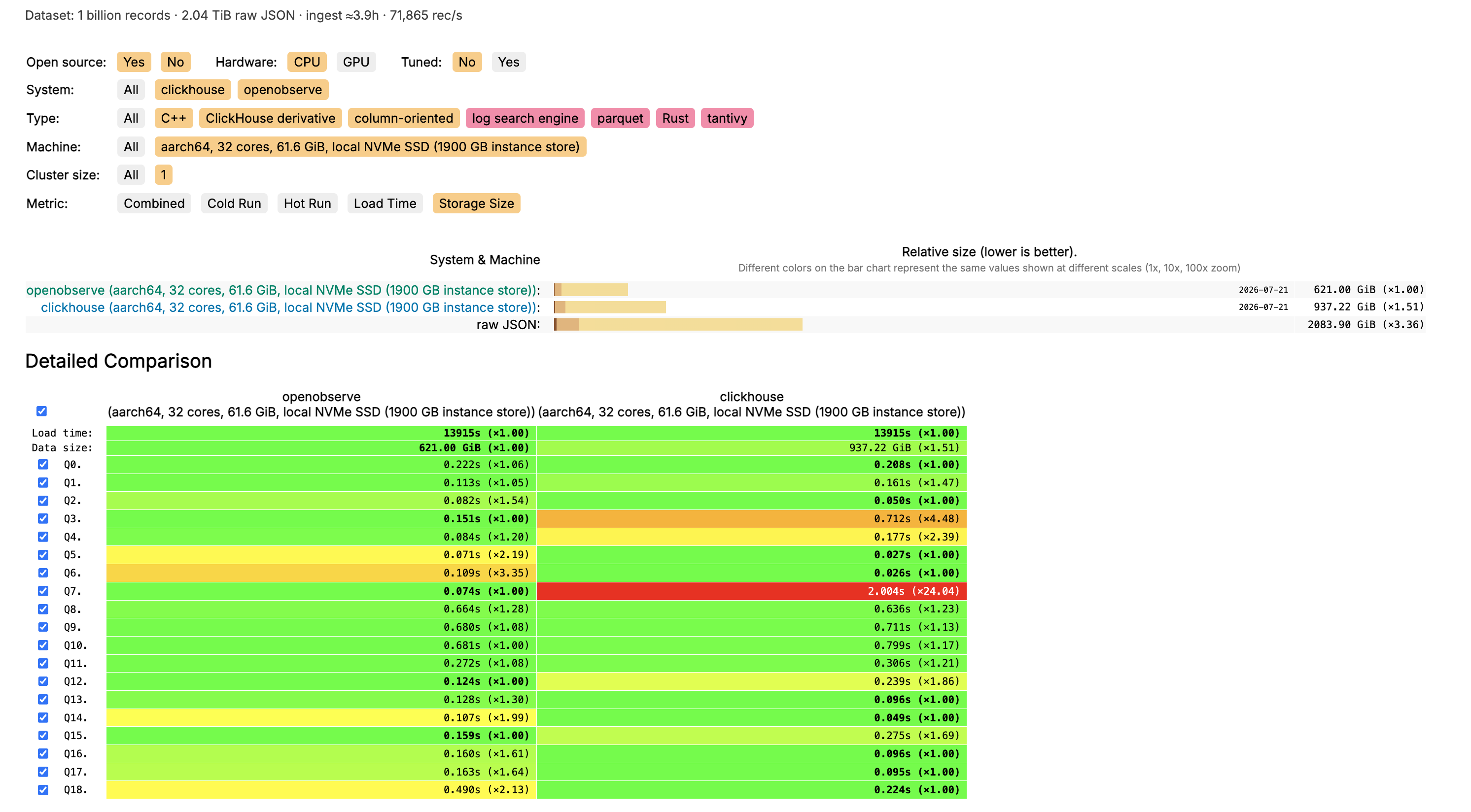
The report's storage view. The multipliers are relative to the smallest footprint, so raw JSON shows 3.36x OpenObserve's total; the compression column in the table divides the other way.
OpenObserve wrote about a third less to disk, and the index cost is nearly the same on both sides. The difference is in the data itself, where OpenObserve's Parquet columns are smaller than ClickHouse's default-codec columns. The honest reading is the caveat from the config section: ClickHouse ran default compression, not the ZSTD(1) plus Delta codecs its own documentation recommends for log data (ClickHouse blog, where they document 14x to 33x compression depending on the ingestion path). A codec-tuned ClickHouse would close much of this gap, so we are not claiming a storage win here. If storage is your deciding factor, set the codecs and measure it yourself. The more important system question is whether object storage is the default durable data layer or an additional storage tier and cache policy to design. This benchmark used local disks for both engines, so it does not turn that architectural difference into a cost result. See our log management tools comparison for how footprint plays out across other backends.
Times below are from the NVMe run: the cold (cache-dropped) run and the warm number, lower is better. This table shows representative queries; the benchmark repository contains all 19.
| Query | OpenObserve cold | OpenObserve warm | ClickHouse cold | ClickHouse warm |
|---|---|---|---|---|
| trace_id count | 714 ms | 58 ms | ✅ 677 ms | ✅ 51 ms |
| span_id count | ✅ 278 ms | 58 ms | 496 ms | ✅ 49 ms |
| rare token count | 151 ms | 59 ms | ✅ 122 ms | ✅ 26 ms |
| "failed" count (common token) | ✅ 217 ms | ✅ 129 ms | 1.19 s | 553 ms |
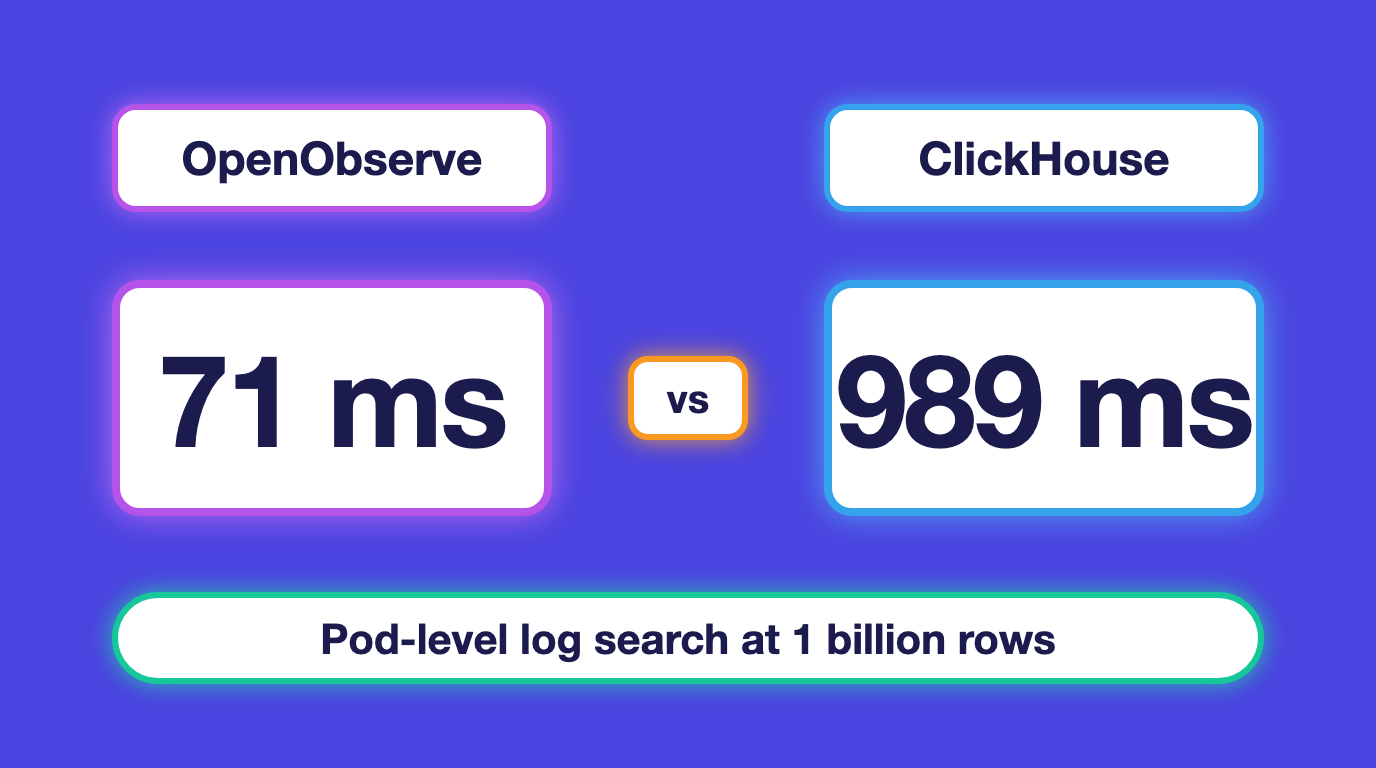
| pod_name count | ✅ 82 ms | ✅ 71 ms | 5.05 s | 989 ms |
| histogram, 1h buckets | ✅ 673 ms | 661 ms | 1.15 s | ✅ 464 ms |
| top-N namespaces | ✅ 1.05 s | 555 ms | 1.39 s | ✅ 485 ms |
| filtered histogram | ✅ 715 ms | 670 ms | 1.19 s | ✅ 668 ms |
trace_id SELECT * |
✅ 514 ms | 191 ms | 732 ms | ✅ 163 ms |
"failed" SELECT * |
196 ms | 78 ms | ✅ 80 ms | ✅ 39 ms |
pod_name SELECT * |
943 ms | 339 ms | ✅ 508 ms | ✅ 130 ms |
✅ marks the faster engine in each cold pair and each warm pair. Across all 19 queries on NVMe, ClickHouse was faster on 15 of the warm runs and OpenObserve on 4; cold, OpenObserve was faster on 10 and ClickHouse on 9. The warm filtered histogram is effectively a tie at 668 ms against 670 ms.
Those win counts need reading together, because they describe different shapes of victory. ClickHouse's warm wins are mostly tens of milliseconds: 51 ms against 58 ms on the trace id, 49 ms against 58 ms on the span id, margins nobody feels in a log viewer. OpenObserve's wins are measured in multiples, and they land on the two query shapes that hurt most in production. A common token, "failed", defeats ClickHouse's text-index pruning. The rare request id lives in a handful of data blocks, so the index skips nearly everything; a token that recurs throughout a billion rows sits in essentially every block, leaving nothing to skip, and ClickHouse pays scan-level cost: 553 ms warm against OpenObserve's 129 ms, a 4.3x gap. A pod name whose matches are scattered across the full time range does the same to the bloom filter: 989 ms warm against 71 ms, 13.9x, and 5.05 seconds against 82 ms cold. A bloom filter tells ClickHouse which granules might contain a value, and with matches spread across a billion rows that still means touching a lot of granules. OpenObserve's inverted index points at the rows directly, so its latency depends on the result, not on how the matches are scattered. Our query performance tuning docs go deeper on why the index paths behave this way.
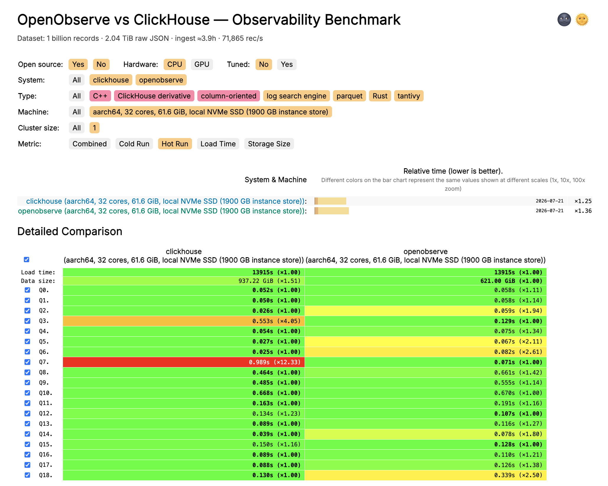
One note on reading that chart: the multipliers in it follow the ClickBench convention of adding 10 ms to both sides before dividing, which damps the ratios on very fast queries. That is why it labels the warm pod-name gap 12.33x while the raw numbers (989 ms against 71 ms) divide out to 13.9x. We quote the raw ratio in this post and left the chart on the standard convention.
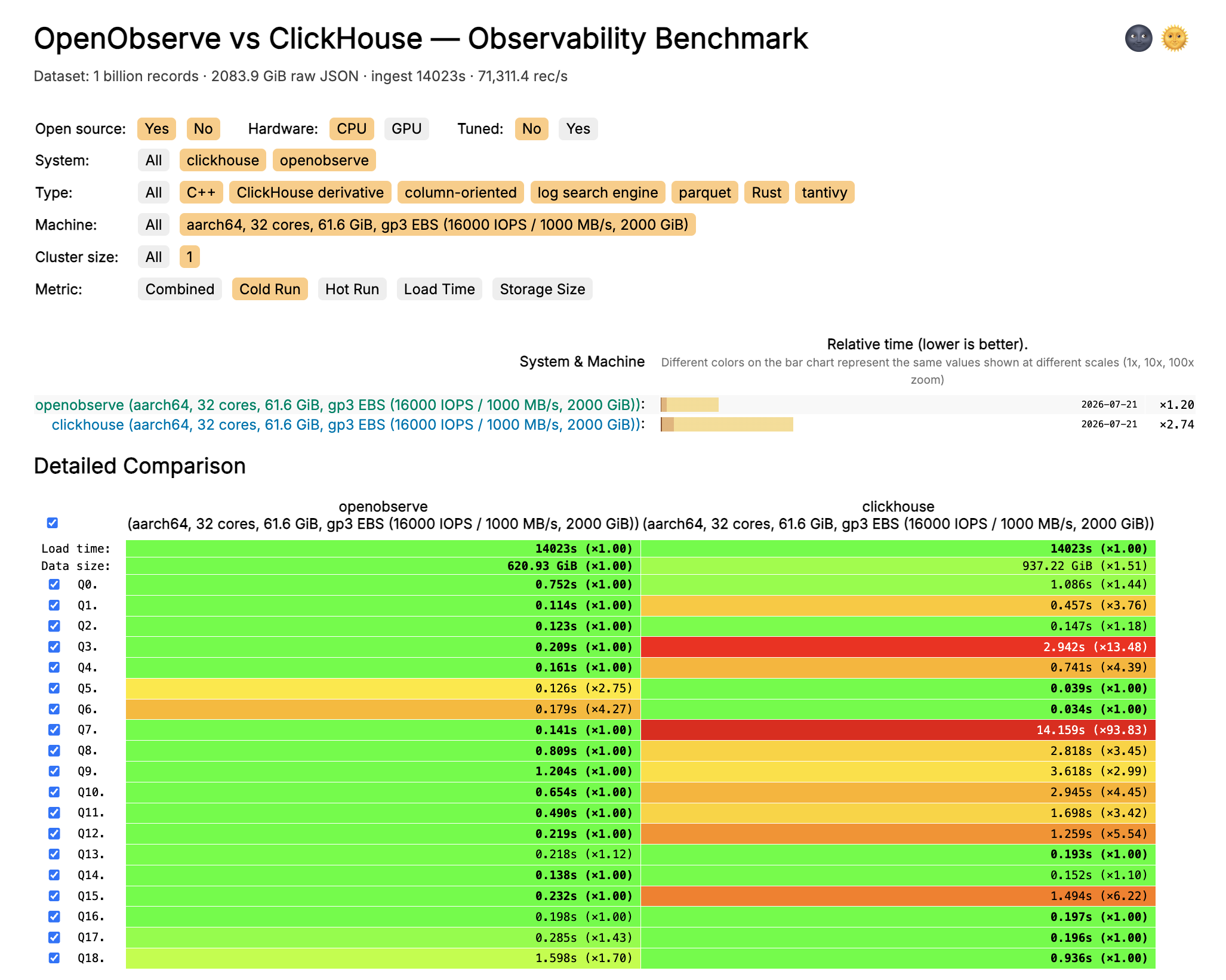
We ran the identical benchmark a second time on gp3 EBS, provisioned at gp3's maximum 16,000 IOPS and 1000 MB/s, so this is gp3 at its best. Warm latencies barely changed for either engine: warm queries are answered from RAM and indexes, and the warm win count stayed 15 to 4 for ClickHouse. Cold is a different story.
| Query (cold run) | ClickHouse on NVMe | ClickHouse on gp3 | ClickHouse change | OpenObserve on NVMe | OpenObserve on gp3 |
|---|---|---|---|---|---|
| pod_name count | 5.05 s | 14.16 s | 2.8x slower | 82 ms | 141 ms |
| "failed" count | 1.19 s | 2.94 s | 2.5x slower | 217 ms | 209 ms |
| histogram, 1h buckets | 1.15 s | 2.82 s | 2.4x slower | 673 ms | 809 ms |
| top-N namespaces | 1.39 s | 3.62 s | 2.6x slower | 1.05 s | 1.20 s |
| filtered histogram | 1.19 s | 2.95 s | 2.5x slower | 715 ms | 654 ms |
span_id SELECT * |
552 ms | 1.26 s | 2.3x slower | 175 ms | 219 ms |
compound SELECT * |
651 ms | 1.49 s | 2.3x slower | 253 ms | 232 ms |
The seven cold queries in the table got 2.3x to 2.8x slower moving from NVMe to gp3, because their cold path reads enough data to be bound by the disk. Averaged across all 19 queries (geometric mean), the slower disk cost ClickHouse 1.8x on cold runs and cost OpenObserve 3 percent. OpenObserve's cold latencies changed little in either direction, because its index reads touch little data, so the disk tier barely shows up: several improved, and its one sizable regression was the pod-name row fetch, 943 ms to 1.60 s. The extreme is the pod-name count: 141 ms against 14.16 seconds, roughly a 100x gap on the exact query an engineer runs first during an incident. Cold overall on gp3, OpenObserve was faster on 13 of 19 queries; ClickHouse kept 6: two token counts, three token row fetches, and the pod-name row fetch (936 ms against OpenObserve's 1.60 s, OpenObserve's worst cold query on gp3).
This matters because incident investigation often reaches data that is not already cached. The first query against last night's logs is a cold query, and on commodity cloud disks the two engines give you very different first answers: on gp3, OpenObserve's cold latencies stayed between 114 ms and 1.60 s across all 19 queries, while ClickHouse's ranged from 34 ms to 14.16 s.
In OpenObserve, searching text is one function on data that was indexed automatically.
-- OpenObserve: find a request id anywhere in the message
SELECT count(*) FROM k8s_logs WHERE match_all('474dbfe4c65a971176ae239869a6ba47');
In ClickHouse the same search works, but only because we added the text() index in the schema above, and you query it with the matching function.
-- ClickHouse: same needle, through the text() index
SELECT count() FROM k8s_logs
WHERE hasAnyTokens(message, ['474dbfe4c65a971176ae239869a6ba47']);
Both found the needle in a billion rows fast, and warm, ClickHouse was faster: 26 ms against 59 ms. The difference is setup, not capability: ClickHouse's full-text indexing is something you choose, size, and maintain, while on OpenObserve it is on by default for the fields you mark. And the same text index that wins on a rare token is the one that falls behind by 4.3x when the token is common: indexed search in ClickHouse is sensitive to how often the term appears, where OpenObserve's stays flat.
An honest benchmark reports its losses, and ClickHouse beat OpenObserve in real ways here.
Query performance is the last piece of this decision, not the whole decision. This benchmark asked a narrow question: if a team chooses OpenObserve for its object-storage-first architecture, automatic schema evolution, and integrated observability experience, does it have to accept weak query performance? At a billion rows, the answer was no, with an honest asymmetry. Warm, ClickHouse is faster on most queries by tens of milliseconds; OpenObserve is faster on the heaviest search patterns by multiples. Cold, and especially cold on commodity disks, OpenObserve is the more predictable engine.
The setup was deliberately conservative for that broader claim. ClickHouse ran native MergeTree on local disk, while OpenObserve also ran on local disk even though its cloud-native architecture uses object storage as the durable system of record. That makes the latency comparison reproducible, but it leaves OpenObserve's production storage economics and elasticity out of the result. This is not an S3 performance or total-cost benchmark; it shows that OpenObserve remains competitive even without counting one of the main reasons teams choose it.
The operating model is different too. The ClickHouse table in this test explicitly defined 27 columns and four indexes. Maintaining that optimized schema and index layout as logs gain fields or change shape is part of operating the system. OpenObserve discovers fields, infers their types, and evolves the stream schema during ingestion. ClickHouse gives you a powerful analytical database; OpenObserve gives you an observability product that integrates ingestion, search, dashboards, alerts, and retention across logs, metrics, and traces. A single-node OpenObserve deployment can run as one binary, and the product remains integrated when the infrastructure scales out.
So the practical answer is not "use ClickHouse for histograms and OpenObserve for needle searches." The split is what you are choosing. If you are picking a database engine, ClickHouse can win that contest: analytical SQL, consistently fast warm queries, and a cluster you may already run well. If you are starting an observability platform, the small warm margins matter less than what surrounds them: storage architecture, cost, schema evolution, and the work of building and operating everything around the engine.
For most teams looking for a complete cloud-native observability system, start with OpenObserve. It does not win every query; ClickHouse's warm wins and its row-fetch performance in this benchmark are real. But performance is no longer a reason to give up low-cost object storage, schemas that adapt as logs change, and one integrated product instead of a database around which you still have to assemble the experience.
If automatic schema evolution, built-in indexed search, and an integrated observability experience appeal to you, the fastest way to feel the difference is to point some real logs at it. OpenObserve Cloud gives you ingestion, full-text search, dashboards, and alerting without running the binary yourself, and the same engine is open source if you prefer to self-host. Every schema, query, and install script from this benchmark is in the benchmark repository if you want to rerun it on your own account.


Hengfei Yang is the founding engineer at OpenObserve. He has extensive experience in distributed system development. He is passionate about open source and has interests in traveling, music and photography.
Huaijin Hao is a backend engineer at OpenObserve, focused on building scalable, high-performance distributed systems. He is passionate about cloud-native technologies and open source.
Gorakhnath is a passionate developer advocate, working on bridging the gap between developers and the tools they use. He focuses on building communities and creating content that empowers developers to build better software.