Caught Before It Mattered: How a Slow Latency Drift Almost Became a Black Friday Outage



Ready to get started?
Try OpenObserve Cloud today for more efficient and performant observability.
This is a guest post from the team at DataElicit Solutions, an ISO 27001 certified MSSP that helps organizations design and run their observability and security operations. In it, they share a use case from their work with OpenObserve.
TL;DR
- A routine library upgrade caused a connection pool leak that made p99 latency drift up about 4 ms a day, below every static alert threshold for 18 days.
- A VRL pipeline had already turned a free-text "connection pool wait" warning into a numeric
wait_msfield. - Baseline-compared alerts caught the slope by comparing the last six hours against the same window a week earlier.
- A composite alert combined the log trend and the latency trend into one OpenObserve incident.
- Traces pinpointed the leak, and a 15-line fix shipped 11 days before Black Friday.
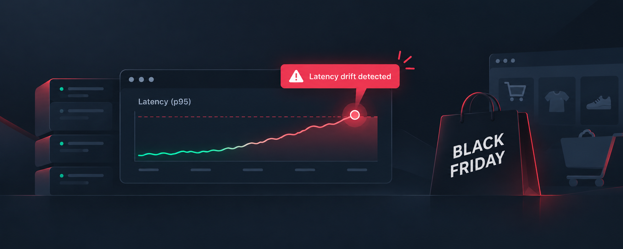
Three weeks before Black Friday, p99 latency on a checkout service had crept up by about four milliseconds a day. No dashboard called that an incident. No static threshold came close to tripping. But compounded daily, against a traffic event that runs at ten times normal load, four milliseconds a day is exactly the kind of thing that becomes an outage on the one day you can least afford one.
This is a composite scenario built from a pattern we see repeatedly across our engagements, not a single client's exact timeline. What follows is how a slow, boring drift became visible before it became a page, and why the telemetry that caught it was already being collected in OpenObserve for entirely unrelated reasons.
The setup: an e-commerce platform and a quiet library upgrade
The environment was an e-commerce platform sending application logs, infrastructure and service metrics, and distributed traces to OpenObserve. None of it was built to catch this specific problem. Metrics existed for capacity planning. Traces existed for latency debugging. Logs existed because that's where errors show up.
Three weeks earlier, a routine library upgrade had changed how a backend service pooled connections to a downstream payment gateway client. Under normal load, the change was invisible: connections still got returned to the pool, just slightly slower on one specific retry path.
Under load, that slowness compounds. Connections held a little longer means fewer are available for the next request, which means more requests wait, which means more connections held a little longer.
What did the telemetry actually show?
Two signals existed, and neither was dramatic on its own:
| Signal | What it showed | Why no alert fired |
|---|---|---|
| Metrics: p99 latency on the payment call | A slow upward slope, day over day | Nowhere near any static threshold, and indistinguishable from noise on any single day's graph |
| Logs: "connection pool wait" warnings | A rising count of non-fatal warnings, every one eventually succeeding on retry | No errors and no failed checkouts, so a standard error-rate alert would never see it |
Neither signal justified a page by itself. A slow latency drift is often just noise. A retried, non-fatal warning is exactly the kind of thing most teams tune their alerts to ignore, for good reason, most of the time.
Where the pipeline made the difference
An OpenObserve Pipeline on the application log stream was already running a VRL function that parsed the wait time out of each "connection pool wait" warning and attached it as a numeric field, instead of leaving it buried in a free-text message. That's what turned "a warning happened" into a trend line: the average wait time, and how fast it was moving.
# Pipeline function on the application log stream
parsed, err = parse_regex(.message, r'connection wait (?P<wait_ms>\d+)ms')

if err == null {
  .wait_ms = to_int!(parsed.wait_ms)
  .is_slow_wait = .wait_ms > 300
} else {
  .is_slow_wait = false
}
With wait_ms as a real numeric field, a scheduled alert could ask a sharper question than any static threshold: is the average wait time over the last six hours meaningfully higher than the same window a week ago? OpenObserve's Compare with Past setting on scheduled alerts makes exactly that comparison, and it's what caught a slope no single-point threshold ever would.
From alert to incident: how a composite alert connected the dots
One alert on a slowly rising average is the kind of thing an on-call engineer might reasonably snooze until morning. This is where a composite alert changed the outcome. It combined the log-based wait-time trend with a second scheduled alert on the metrics stream, which tracked the same week-over-week comparison on p99 latency for the same service.
Neither alert alone was urgent. Both trending up together, on the same service, in the same window, was. OpenObserve correlated them into a single incident with severity and service context attached.
| When | What happened | Signal state |
|---|---|---|
| Days 1-18 | p99 latency drifts, unnoticed | Metric below any static threshold |
| Day 19 | wait_ms trend rises |
Parsed log field, still below threshold |
| Day 19 | Composite alert fires | Incident opened, both trends attached |
| Day 20 | Connection leak patched | Investigated across logs, metrics, and traces, then fixed |
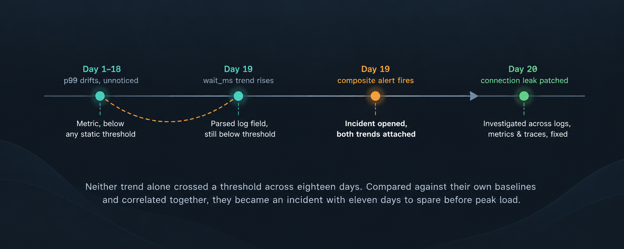
Neither trend alone crossed a threshold across eighteen days. Compared against their own baselines and correlated together, they became an incident with eleven days to spare before peak load.
The investigation: from "checkout is slow" to the root cause
With an incident open and both trends attached, the on-call engineer didn't start from a blank dashboard. Pivoting into traces for the payment call showed exactly where the time was going: a growing span duration around acquiring a connection from the pool, not the payment gateway call itself. That narrowed the search from "checkout is slow" to "connection pooling is slow" in one pivot.
Cross-referencing the timeline against recent deploys pointed at the library upgrade from three weeks earlier. The upgrade had changed how failed retries released their connection back to the pool. It was a leak that only showed up under the intermittent failure rate normal traffic produces occasionally, and that a load test rarely reproduces at the same frequency.
The fix: fifteen lines correcting the release path, deployed eleven days before Black Friday, with p99 latency back to baseline within an hour of rollout.
What would have happened without correlation?
Without the correlation, the drift keeps compounding quietly. Four milliseconds a day is nothing on any single day's dashboard. Eighteen more days of that same drift, arriving at ten times normal traffic on the highest-revenue day of the year, is a connection pool exhausted within minutes of the traffic spike, and a checkout service returning errors during the exact window it can least afford to.
The actual gap: It was never a missing metric or a missing log line. Every signal used here was already being collected for unrelated reasons. The gap was that nothing compared today's slope against last week's baseline, across two signal types, until a pipeline and a composite alert did.
Why the architecture mattered as much as the data
Logs, metrics, and traces lived in one platform with a shared time axis and the same alerting engine. That's what made an eighteen-day slope visible as one story instead of three disconnected graphs someone had to think to compare manually.
A parsed log field, a metric trend, and a trace span all pointed at the same root cause because they could all be queried against the same timeline, by the same person, in one investigation. It's the same gap OpenObserve covers in fixing the logs, traces, and metrics correlation gap.
Lessons from this use case
- Parse the number out of the warning; don't leave it in free text. A wait time, a retry count, or a queue depth buried in a log message is invisible to trend analysis until it's a real field. One VRL function, applied once at ingest, makes it queryable everywhere afterward.
- Alert on trend versus baseline, not just absolute thresholds. A slow-burning drift can stay under any fixed threshold for weeks while still being exactly the kind of problem worth catching early. Comparing against a rolling baseline catches shape, not just magnitude.
- Build composite alerts across signal types for anything that compounds. A latency trend and a warning-count trend, each individually dismissible, become a real signal in combination. If two independently weak trends point at the same service, that combination deserves its own alert.
- Keep deploys on the same timeline as everything else. The fastest part of this investigation was correlating the drift's start date against a known deploy. That's only fast if deploy history is visible next to the telemetry, not filed away in a separate system.
If we had to pick the single highest-leverage thing to replicate, it's the composite, baseline-compared alert, not the parsing. Parsing makes one signal sharper; comparing two independently weak trends against their own history is what surfaces a slow-burning problem before a threshold ever would. For drift detection that doesn't need a manually configured comparison window, OpenObserve also offers built-in anomaly detection.
Further reading
- OpenObserve alerts overview: scheduled, real-time, and composite alerts
- Scheduled alerts: time-window and baseline comparisons
- Pipelines and functions: ingest-time enrichment with VRL
- Incidents in OpenObserve: correlated alerts with severity and service context
- Incident correlation: the complete guide
- How to fix alert fatigue
Conclusion
The lesson underneath this story isn't "watch your latency more closely," though that's true too. It's that most of the telemetry needed to catch a slow-burning problem is probably already flowing somewhere in your environment. The gap is rarely collection. It's whether anything is positioned to compare today against last week, across more than one signal, before the day arrives when the drift finally runs out of room.
Want to try baseline and composite alerts on your own telemetry? Start a free OpenObserve Cloud trial or download self-hosted OpenObserve.
Frequently Asked Questions
About the Author
Tejas Shah

Tejas Shah is Chief Solutions Architect and advisor for SIEM and Observability at DataElicit Solutions, an ISO 27001 certified MSSP and Splunk partner based in India. His work spans SIEM architecture, technical enablement, and managed security operations across the observability ecosystem.
Follow OpenObserve on Google
Add OpenObserve as a preferred source to see more of our articles in Google Search and Top Stories.